4 MRI characteristics and DUX4 molecular signatures
In this chapter, we conduct a validation of the correlation between MRI characteristics and DUX4 signatures, which are represented by six robust DUX4 genes (refer to Appendix(1appendixB-DUX4-baskets-curation)). Additionally, we constructed a logistics regression model using MRI characteristics as predictors to forecast the occurrence of DUX4 of a muscle biopsy.
Noted that the muscle less biopsies (13-0007R and 13-0009R) identified in Chapter 3 might not accurately represent the expression originated from muscle cells. As a result, we excluded them from this DUX4-MRI correlation analysis.
# load libraries
suppressPackageStartupMessages(library(tidyverse))
suppressPackageStartupMessages(library(DESeq2))
suppressPackageStartupMessages(library(writexl))
suppressPackageStartupMessages(library(knitr))
suppressPackageStartupMessages(library(kableExtra))

# load data sets
pkg_dir <- "/Users/cwon2/CompBio/Wellstone_BiLateral_Biopsy"
draft_fig_dir <- file.path(pkg_dir, "manuscript", "figures")
load(file.path(pkg_dir, "data", "comprehensive_df.rda"))
load(file.path(pkg_dir, "data", "bilat_dds.rda"))
load(file.path(pkg_dir, "data", "all_baskets.rda"))

dds <- bilat_dds[, !bilat_dds$sample_id %in% c("13-0007R", "13-0009R")]
# tidy annotation
anno_gencode35 <- as.data.frame(rowData(dds)) %>%
  rownames_to_column(var="gene_id") %>% #BiLat study using Gencode 35
  dplyr::mutate(ens_id=str_replace(gene_id, "\\..*", ""))

# color palate
library(wesanderson)
pal <- wes_palette("Darjeeling1", n=5)
stir_pal <- c("STIR-" = pal[5], "STIR+"= pal[1])
cntr_pal <- pal[2]
4.1 STIR status and DUX4 signatures
The score of DUX4 signatures here is represented by the sum of log10 TPM expression of six robust DUX4 genes (\(\sum_{i=1}^6 \log_{10}(TPM_i+1)\)). The six robust genes are ZSCAN4, CCNA1, PRAMEF5, KHDC1L, H3Y1, and MBD3L2.
comprehensive_df %>% drop_na(`DUX4-M6-logSum`) %>%
  dplyr::filter(!sample_id %in% c("13-0007R", "13-0009R")) %>%
  group_by(STIR_status) %>%
  summarise(`DUX4 score (mean of log sum)` = mean(`DUX4-M6-logSum`)) %>%
  kbl(caption="Mean values of DUX4 scores (based on DUX4-M6 basket) in STIR+ and STIR- biopsies.") %>%
kable_styling()| STIR_status | DUX4 score (mean of log sum) |
|---|---|
| STIR+ | 3.0286217 |
| STIR- | 0.4073134 |
The mean difference of DUX4 scores in STIR+ and STIR- groups is significantly greater than 0 with Wilcox \(p\)-value \(7e-10\).
dux4_list <- comprehensive_df %>% drop_na(`DUX4-M6-logSum`) %>%
  dplyr::filter(!sample_id %in% c("13-0007R", "13-0009R")) %>%
  group_by(STIR_status) %>%
  group_map(~ pull(.x, `DUX4-M6-logSum`))

wilcox.test(dux4_list[[1]], dux4_list[[2]])
#>
#>  Wilcoxon rank sum exact test
#>
#> data:  dux4_list[[1]] and dux4_list[[2]]
#> W = 815, p-value = 7.315e-10
#> alternative hypothesis: true location shift is not equal to 0
4.2 Logistics prediction of DUX4 signature occurrence
4.2.1 Scheme 1: use random forest traning model based on DUX4 M6 basket
The initial approach utilized a random forest training model derived from the longitudinal cohort featuring six DUX4 basket genes. We applied this machine learning model to classify DUX4+ and DUX4- groups within the bilateral samples. As a result, we identified 60% and 95% of the STIR- and STIR+ samples, respectively, as DUX4+.
# MH_fit$M6 is built on comparing controls and Moderate+IG-high+High
id <- all_baskets[["DUX4-M6"]]$gencode_v35
df_logTPM <- log10(assays(dds[id])[["TPM"]] + 1) %>% t(.) %>%
      as.data.frame() %>%
      tibble::add_column(pheno_type = factor("FSHD",
                                             levels=c("Control",
                                                      "FSHD"))) %>%
      rename_with(~ str_replace(.x, "\\..*", ""), starts_with("ENSG"))
MH_fit <- get(load(file.path(pkg_dir, "data", "MH_fit.rda")))$M6

predict_M6 <- predict(MH_fit$rf, newdata=df_logTPM) %>%
  as.data.frame() %>% dplyr::rename(rfM6_fit = ".") %>%
  tibble::add_column(sample_id = str_replace(rownames(df_logTPM),
                                     "_.*", ""))
data <- predict_M6 %>%
  left_join(comprehensive_df, by="sample_id") %>%
  drop_na(STIR_status)
# how many STIR- and STIR+ on Control (DUX4-) and FSHD (DUX4+)
data %>% group_by(STIR_status) %>%
  summarise(`DUX4-` = sum(rfM6_fit=="Control"),
            `DUX4+` = sum(rfM6_fit == "FSHD")) %>%
knitr::kable(caption="STIR+ and - distribution on the DUX4+/- group.")| STIR_status | DUX4- | DUX4+ |
|---|---|---|
| STIR+ | 1 | 21 |
| STIR- | 12 | 28 |
data %>% group_by(rfM6_fit) %>%
  summarize(average_DUX4_score = mean(`DUX4-M6-logSum`),
            min_DUX4_score = min(`DUX4-M6-logSum`),
            max_DUX4_score = max(`DUX4-M6-logSum`))
#> # A tibble: 2 × 4
#>   rfM6_fit average_DUX4_score min_DUX4_score max_DUX4_score
#>   <fct>                 <dbl>          <dbl>          <dbl>
#> 1 Control              0.0408         0.0260         0.0668
#> 2 FSHD                 1.68           0.0856         6.05
The general linear model depicted that STIR status was key to the association to DUX4 signatures whereas fat infiltration or fraction presented less solid evident of direct association (p-value=0.3).
The code chunk below applies the logistic regression using a fat infiltration percent and STIR status as predictors and outcome of DUX4 signature occurrence predicted by random forest:
# include random forest fitting model (M6) and threshold
data <- predict_M6 %>%
  left_join(comprehensive_df, by="sample_id") %>%
  drop_na(STIR_status)
fat_stir_logit <- glm(rfM6_fit ~ Fat_Infilt_Percent + STIR_status,
                      data = data, family = "binomial")
summary(fat_stir_logit)
#>
#> Call:
#> glm(formula = rfM6_fit ~ Fat_Infilt_Percent + STIR_status, family = "binomial",
#>     data = data)
#>
#> Deviance Residuals:
#>     Min       1Q   Median       3Q      Max
#> -2.1852   0.0535   0.5196   0.8248   0.9502
#>
#> Coefficients:
#>                    Estimate Std. Error z value Pr(>|z|)
#> (Intercept)          0.2206     0.6796   0.325    0.746
#> Fat_Infilt_Percent   7.2107     6.8399   1.054    0.292
#> STIR_statusSTIR+     0.8861     1.2679   0.699    0.485
#>
#> (Dispersion parameter for binomial family taken to be 1)
#>
#>     Null deviance: 63.678  on 61  degrees of freedom
#> Residual deviance: 55.200  on 59  degrees of freedom
#> AIC: 61.2
#>
#> Number of Fisher Scoring iterations: 7
df_scheme1 <- data.frame(Fat_Infilt_Percent = rep(seq(0, 0.8, by=0.01), 2),
                 STIR_status = rep(c("STIR-", "STIR+"),
                                  each=length(seq(0, 0.8, by=0.01))))
df_scheme1$prob <- predict(fat_stir_logit, newdata = df_scheme1, type = "response")

ggplot(df_scheme1, aes(x=Fat_Infilt_Percent, y=prob, group=STIR_status,
               color=STIR_status)) +
  geom_line() +
  scale_color_manual(values = stir_pal) +
  theme_minimal() +
  theme(legend.position = "top", axis.title.y=element_text(size=10),
        plot.title=element_text(size=12, hjust=0.5),
        plot.subtitle=element_text(size=10, hjust=0.5)) +
  labs(title="Logistic prediction for DUX4+ occurrance",
       subtitle = "DUX4+/- classified by ML model",
        y="probility of DUX4 signature occurence",
        x="whole muscle fat percent") +
  scale_x_continuous(breaks=seq(0, 0.8, by=0.2)) +
  scale_y_continuous(breaks=seq(0, 1, by=0.1))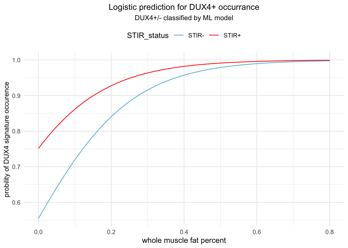
Figure 4.1: Prediction of DUX4 + ocurrence modeled by linear combination of STIR_status and FAT_Infilt_Percent. The red linepresents STIR+ and blue STIR-.
4.2.2 Scheme 2: Binary outcome using DUX4 score > 0.5
We use the DUX4 score defined by the accumulated log(TPM+1) over the six genes of the DUX4 basket. Then use whole muscle fat percent and STIR status as predictor to infer the occurrence of DUX4 score > 0.5. The reason we chose 0.5 threshold was because TPM=0.2 is a conventional threshold to call whether a gene is expressed and sum of six genes with expressed level is approximately 0.5: \(\sum_1^6 log_{10}(0.2 + 1) \approx 0.5\).
NOTE: Predictions for 13-0007R and 13-0009R are excluded.
# include random forest fitting model (M6) and threshold
data <- comprehensive_df %>% drop_na(STIR_status, `DUX4-M6-logSum`) %>%
  dplyr::select(sample_id, `DUX4-M6-logSum`, Fat_Infilt_Percent, STIR_status) %>%
  dplyr::filter(!sample_id %in% c("13-0007R", "13-0009R")) %>%
  dplyr::mutate(`DUX4-M6-logSum-positive`= if_else(`DUX4-M6-logSum` < 0.5,
                                                   "Control-like", "DUX4+")) %>%
  dplyr::mutate(`DUX4-M6-logSum-positive`=factor(`DUX4-M6-logSum-positive`))

## how many STIR- are control-like (DUX4 score < 0.5) and
##how many STIR+ are DUX4+ (DUX4 >= 0.5)
data %>% group_by(STIR_status) %>%
  summarise(`DUX4 < 0.5`=sum(`DUX4-M6-logSum-positive` == "Control-like"),
            `DUX4 > 0.5`= sum(`DUX4-M6-logSum-positive` == "DUX4+")) %>%
  kbl(caption = "Number of STIR- and STIR+ in the DUX4 < 0.5 and DUX4 >=0.5 group.") %>%
kable_styling()| STIR_status | DUX4 < 0.5 | DUX4 > 0.5 |
|---|---|---|
| STIR+ | 1 | 21 |
| STIR- | 31 | 9 |
In this case, the general linear model depicted that STIR status was key to the association to DUX4 signatures whereas fat infiltration or fraction presented less solid evident of direct association (p-value=0.3). Summary of the logistic regression statistics:
## logistic prediction
fat_stir_logit_2 <- glm(`DUX4-M6-logSum-positive` ~ Fat_Infilt_Percent + STIR_status,
                        data = data, family = "binomial")
summary(fat_stir_logit_2)
#>
#> Call:
#> glm(formula = `DUX4-M6-logSum-positive` ~ Fat_Infilt_Percent +
#>     STIR_status, family = "binomial", data = data)
#>
#> Deviance Residuals:
#>     Min       1Q   Median       3Q      Max
#> -2.1838  -0.7054  -0.5871   0.3009   1.8516
#>
#> Coefficients:
#>                    Estimate Std. Error z value Pr(>|z|)
#> (Intercept)         -1.9431     0.7751  -2.507   0.0122 *
#> Fat_Infilt_Percent   7.8039     7.2899   1.071   0.2844
#> STIR_statusSTIR+     2.9489     1.2501   2.359   0.0183 *
#> ---
#> Signif. codes:
#> 0 '***' 0.001 '**' 0.01 '*' 0.05 '.' 0.1 ' ' 1
#>
#> (Dispersion parameter for binomial family taken to be 1)
#>
#>     Null deviance: 85.886  on 61  degrees of freedom
#> Residual deviance: 48.859  on 59  degrees of freedom
#> AIC: 54.859
#>
#> Number of Fisher Scoring iterations: 7
df_scheme2 <- data.frame(Fat_Infilt_Percent = rep(seq(0, 0.8, by=0.01), 2),
                 STIR_status = rep(c("STIR-", "STIR+"),
                                  each=length(seq(0, 0.8, by=0.01))))
df_scheme2$prob = predict(fat_stir_logit_2, newdata = df_scheme2, type = "response")
fat_logit <- glm(`DUX4-M6-logSum-positive` ~ Fat_Infilt_Percent,
                 data = data, family = "binomial")
df_fat_logit <- data.frame(Fat_Infilt_Percent = seq(0, 0.8, by=0.01))
df_fat_logit$prob <- predict(fat_logit, newdata = df_fat_logit, type="response")
# add a logistic model without STIT
# viz
ggplot(df_scheme2, aes(x=Fat_Infilt_Percent, y=prob, group=STIR_status,
                       color=STIR_status)) +
  geom_line() +
  geom_line(data=df_fat_logit,
            aes(x=Fat_Infilt_Percent, y=prob), color="gray75",
            linetype="dashed", inherit.aes=FALSE) +
  scale_color_manual(values = stir_pal) +
  theme_minimal() +
  theme(legend.position = "none",
        axis.title.x = element_text(size=9),
        axis.title.y = element_text(size=9),
        plot.subtitle = element_text(size=9, color="grey20", hjust=0.5),
        plot.title=element_text(hjust=0.5, size=10)) +
  labs(title="Logistic regression",
       subtitle="Occurrence of DUX4 score > 0.5",
        y="probility",
        x="whole muscle fat percent") +
  scale_x_continuous(breaks=seq(0, 0.8, by=0.2)) +
  scale_y_continuous(breaks=seq(0, 1, by=0.2)) +
  geom_segment(aes(x = 0.13, y = 0.80, xend = 0.11, yend = 0.84),
               color=stir_pal["STIR+"],
               arrow = arrow(length = unit(0.1, "cm"))) +
  annotate("text", x=0.14, y=0.80, hjust=0, vjust=1, label="STIR+", size=2.5,
           color=stir_pal["STIR+"]) +
  geom_segment(aes(x = 0.23, y = 0.35, xend = 0.21, yend = 0.39),
               color=stir_pal["STIR-"],
               arrow = arrow(length = unit(0.1, "cm"))) +
  annotate("text", x=0.24, y=0.35, hjust=0, vjust=1, label="STIR-", size=2.5,
           color=stir_pal["STIR-"])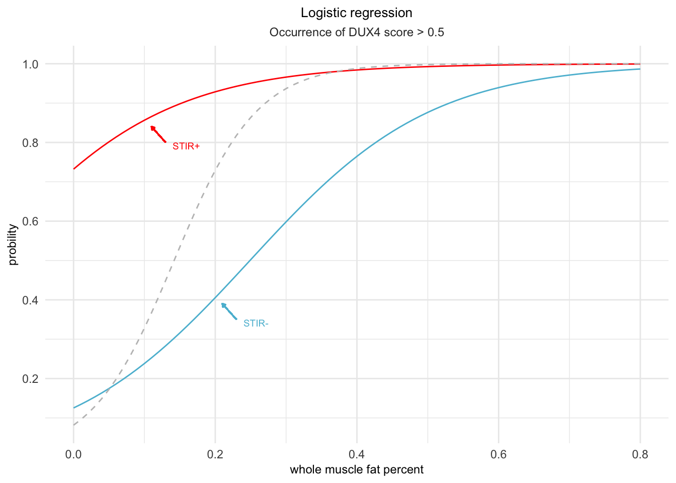
Figure 4.2: A logistic prediction model was used to forecast the likelihood of a DUX4 score greater than or equal to 0.5. The grey dashed line represents the forecast made solely on the basis of fat percentage as the predictor.
4.2.3 Use logistic regression to predict the Moderate+ occurrence
Here, we made the logistics prediction of Moderate+ occurrence based on a random forest model constructed from 30 basket genes that distinguish between control and moderate+IG-high+high FSHD cases. Although the STIR status has a slight impact on the prediction, it is not significant.
# use logistics to predict the Moderate+ occurrence (outcome model built upon)
# six basket;
# take away: fat infiltration percent is critical in determining the probability of the outcome, whereas STIR_status is not

comprehensive_df %>% group_by(STIR_status) %>%
   summarise(`Control-like`=sum(class=="Control-like", na.rm=TRUE),
             `Moderate+`=sum(class=="Moderate+", na.rm=TRUE),
             `Muscle-Low` = sum(class=="Muscle-Low", na.rm=TRUE)) %>%
  kbl() %>%
kable_styling()| STIR_status | Control-like | Moderate+ | Muscle-Low |
|---|---|---|---|
| STIR+ | 2 | 20 | 1 |
| STIR- | 15 | 25 | 1 |
# randomForest.Fit is ML traning model based on six basket genes and
# the longitudinal samples
load(file.path(pkg_dir, "data", "bilat_MLpredict.rda"))
data <- comprehensive_df %>%
  left_join(dplyr::select(bilat_MLpredict, -class), by="sample_id") %>%
  drop_na(randomForest.fit)

fat_stir_logit_3 <- glm(randomForest.fit ~ Fat_Infilt_Percent + STIR_status,
                        data = data, family = "binomial")
summary(fat_stir_logit_3)
#>
#> Call:
#> glm(formula = randomForest.fit ~ Fat_Infilt_Percent + STIR_status,
#>     family = "binomial", data = data)
#>
#> Deviance Residuals:
#>     Min       1Q   Median       3Q      Max
#> -1.8231  -1.2550   0.4110   0.9434   1.1812
#>
#> Coefficients:
#>                    Estimate Std. Error z value Pr(>|z|)
#> (Intercept)         -0.3331     0.6417  -0.519    0.604
#> Fat_Infilt_Percent   9.6883     6.4148   1.510    0.131
#> STIR_statusSTIR+     0.1928     1.0038   0.192    0.848
#>
#> (Dispersion parameter for binomial family taken to be 1)
#>
#>     Null deviance: 72.836  on 61  degrees of freedom
#> Residual deviance: 61.901  on 59  degrees of freedom
#> AIC: 67.901
#>
#> Number of Fisher Scoring iterations: 7

df_scheme3 <- data.frame(Fat_Infilt_Percent = rep(seq(0, 0.8, by=0.01), 2),
                 STIR_status = rep(c("STIR-", "STIR+"),
                                   each=length(seq(0, 0.8, by=0.01))))
df_scheme3$prob <- predict(fat_stir_logit_3, newdata = df_scheme3, type = "response")

ggplot(df_scheme3, aes(x=Fat_Infilt_Percent, y=prob, group=STIR_status,
                       color=STIR_status)) +
  geom_line() +
  scale_color_manual(values = stir_pal) +
  theme_minimal() +
  theme(legend.position = "none",
        plot.title=element_text(hjust=0.5)) +
  labs(title="Logistic prediction III on Moderate+ occurrence",
        y="Probility of Moderate+ occurrence",
        x="fat infiltration percent") +
  scale_x_continuous(breaks=seq(0, 1, by=0.2))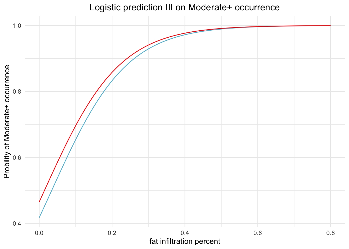
Figure 4.3: Logistic prediction for occurrance of Moderate+. using whole muscle fat percent and STIR status.
df_scheme1 %>%
  left_join(df_scheme2, by=c("Fat_Infilt_Percent", "STIR_status"),
            suffix=c(".scheme1", ".scheme2")) %>%
  left_join(df_scheme3, by=c("Fat_Infilt_Percent", "STIR_status")) %>%
  dplyr::rename(`rfFit Moderare+`=prob, `rfFit DUX4+`=prob.scheme1,
                `threshold DUX4+`=prob.scheme2) %>%
  gather(key=scheme, value=prob, -Fat_Infilt_Percent, -STIR_status) %>%
  #dplyr::mutate(group=paste0(STIR_status, scheme)) %>%
  ggplot(aes(x=Fat_Infilt_Percent, y=prob, group=scheme,
                       color=scheme)) +
  geom_line() +
  #scale_color_manual(values = stir_pal) +
  facet_wrap(~ STIR_status,  nrow=1) +
  theme_minimal() +
  theme(#legend.position = "bottom",
        plot.title=element_text(hjust=0.5)) +
  labs(title="Logistic predictions using three shemes",
        y="Probility of DUX4+ or Moderate+ occurrence",
        x="fat infiltration percent") +
  scale_x_continuous(breaks=seq(0, 1, by=0.2))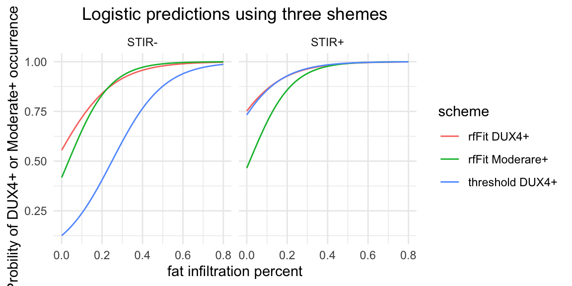
Figure 4.4: Logistic repression for three different classification shemes