3 Transcript-based accessment for muscle content
Characterizing muscle, blood and fat markers expression levels is an important aspect in subsequent analysis of RNA-seq experiments conducted on muscle biopsies. The previous longitudinal and current biolateral studied identified a strong correlation between DUX4 and inflammatory/complement/IG signatures. However, low muscle content biopsies exhibit non-coherent correlation—undetectable-to-low DUX4-targeted expression and elevated inflammatory/ECM complement/IG signatures. We proposed that low muscle biopsies may not primarily reflect the expression of muscle cells but could originated from fat or immune infiltrates cells (see Chapter 8). Hereby we suggested to incorporate three key characteristics to help identify the outlier muscle biopsies lacking muscle content:
Muscle content distribution: Examine the distribution by TPM in three muscle marker genes (ACTA1, TNNT3, MYH1), as well as blood and fat markers. Pay particular attention to samples falling within the lower 3% percentile in muscle markers among the control and other biopsies. Do they show elevated levels in fat or blood markers?
Non-coherent correlation between DUX4 and other disease signatures: the distinctive features in low muscle content biopsies exhibit marker low-to-undetectable DUX4-targeted expression and elevated levels in inflammatory/ECM complement/IG signatures.
Outlier confirmation: Use PCA to observe the muscel biopsies exhibiting low muscle content (i) and properties in (ii) form a cluster distanced from other samples.
3.1 Muscle, blood and fat content distribution
Before performing downstream analysis, we proposed a checkpoint on muscle properties on three transcript-based contents: blood (HBA1, HBA2, and HBB), fat (FASN, LEP, and SCD), and muscle (ACTA1, TNNT3, MYH1), each of which was characterized by a score of average scaled transcripts per million (TPM) — \(\frac{1}{n} \Sigma_{i=1}^{n} \log_{10}(TPM+1)\).
library(DESeq2)
library(tidyverse)
library(ggrepel)
library(pheatmap)
library(wesanderson)

pkg_dir <- "/Users/cwon2/CompBio/Wellstone_BiLateral_Biopsy"
fig_dir <- file.path(pkg_dir, "figures")
# the following script loads bilat_dds, anno_gencode35, longitudinal_dds, anno_ens88
source(file.path(pkg_dir, "scripts", "load_variables_and_datasets.R"))
markers <- tibble(cell_type=c(rep("blood", 3),
                              rep("fat", 3),
                              rep("muscle", 3)),
                  gene_name=c("HBA1", "HBA2", "HBB",
                              "FASN", "LEP", "SCD",
                              "ACTA1", "TNNT3", "MYH1"))  %>%
  dplyr::mutate(cell_type = factor(cell_type)) %>%
  dplyr::left_join(anno_gencode35, by="gene_name")

celltype_tpm <- sapply(levels(markers$cell_type), function(type) {
   id <- markers %>% dplyr::filter(cell_type == type) %>%
      pull(gencode35_id)
   sub <- bilat_dds[id]
   tpm_score <- colSums(log10(assays(sub)[["TPM"]]+1))
}) %>% as.data.frame() %>%
  rownames_to_column(var="sample_name")

blood_fat_muscle_content <- celltype_tpm
3.1.1 Bilateral cohort
Figure 3.1 displays the density and quantile plots of the blood, fat and muscle scores. The gray area present 0 - 97% quantile in fat and blood and 3 - 100% in muscle. Sample 13-0009R and 13-0007R are in the lower 3% quantile in the muscle scores and upper 97% quantile in fat.
data <- blood_fat_muscle_content  %>%
  gather(key=cell_type, value=TPM, -sample_name)  %>%
  dplyr::mutate(cell_type = factor(cell_type))
mark_label <- data %>%
  dplyr::filter(sample_name %in% c("13-0009R", "13-0007R", "32-0020R", "32-0029R")) %>%
  dplyr::filter(!(sample_name %in% c("13-0009R", "13-0007R") & cell_type == "blood")) %>%
  dplyr::filter(!(sample_name %in% c("32-0020R", "32-0029R") &
                                       cell_type %in% c("fat", "muscle")))
# qunatile for each of the cell type content
df_quantile <- data %>% group_by(cell_type) %>%
  summarise(q0 = quantile(TPM, probs=seq(0, 1, 0.01))["0%"],
            q3 = quantile(TPM, probs=seq(0, 1, 0.01))["3%"],
            q97 = quantile(TPM, probs=seq(0, 1, 0.01))["97%"],
            q100 = quantile(TPM, probs=seq(0, 1, 0.01))["100%"]) %>% as.data.frame()
df_rect <- data.frame(cell_type = df_quantile$cell_type,
                      x1 = c(0, 0, df_quantile[3, 3]),
                      x2 = c(df_quantile[1:2, 4], Inf))

ggplot(data, aes(x=TPM)) +
  geom_density() +
  facet_wrap(~cell_type, scales="free_x") +
  theme_bw() +
  theme(panel.grid.minor.x = element_blank(), panel.grid.minor.y = element_blank(),
        panel.grid.major.x = element_blank(), panel.grid.major.y = element_blank(),
        strip.background =element_rect(fill="transparent")) +
  geom_jitter(aes(x=TPM, y=0), size=1, height=0.01) +
  geom_text_repel(data=mark_label, aes(y=0, label=sample_name),
                  size=2.5, color="gray20",
                  min.segment.length = unit(0, 'lines'),
                  nudge_y = .1) +
  geom_rect(data = df_rect, fill="grey50", alpha=0.2,
            aes(xmin = x1, xmax = x2, ymin = -Inf, ymax = Inf), inherit.aes = FALSE) +
labs(x=latex2exp::TeX("RNA-seq cell type content ($\\Sigma \\log_{10}( TPM+1)$"), y="density") 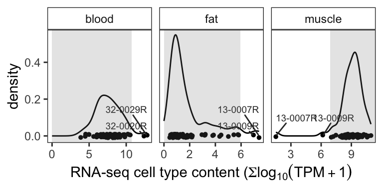
Figure 3.1: Density plot of blood, fat, and muscle marker expression levels. Grey areas present the 0 - 97% (fat and blood) or 3 - 100% (muscle) quantile regions
3.1.2 Muscle content in the bilateral and longitudinal cohorts
markers_ens88 <- tibble(marker_type=c(rep("blood", 3), rep("fat", 3),
                                      rep("muscle", 3)),
                  gene_name=c("HBA1", "HBA2", "HBB",
                              "FASN", "LEP", "SCD",
                              "ACTA1", "TNNT3", "MYH1"))  %>%
  dplyr::mutate(marker_type = factor(marker_type)) %>%
  left_join(anno_ens88, by="gene_name")


markertype_tpm_longi <- sapply(levels(markers_ens88$marker_type), function(type) {
   id <- markers_ens88 %>% dplyr::filter(marker_type == type) %>%
      pull(ens88_id)
   sub <- longitudinal_dds[id]
   tpm_score <- colSums(log10(assays(sub)[["TPM"]]+1))
}) %>% as.data.frame() %>%
  rownames_to_column(var="sample_name") %>%
  add_column(pheno_type = longitudinal_dds$pheno_type,
             classes = longitudinal_dds$cluster)

tmp_longi <- markertype_tpm_longi %>%
  dplyr::mutate(study = if_else(pheno_type=="FSHD", "Longitudinal", "Historical control")) %>%
  dplyr::mutate(group = if_else(classes == "Muscle-Low", "Muscle-Low", "others")) %>%
  dplyr::select(-pheno_type, -classes)

tmp_rbind <- blood_fat_muscle_content %>%
  #dplyr::select(-RNA_sample_id) %>%
  dplyr::relocate(sample_name, .before=blood) %>%
  dplyr::mutate(study = "Bilat") %>%
  dplyr::mutate(group = if_else(sample_name %in% c("13-0007R", "13-0009R"), "Muscle-Low", "others")) %>%
  bind_rows(tmp_longi) %>%
  gather(key=type, value=TPM, -sample_name, -study, -group) %>%
  dplyr::filter(type=="muscle") %>%
  dplyr::mutate(study = factor(study, levels=c("Historical control", "Longitudinal", "Bilat")))

mark_label <- tmp_rbind %>%
  dplyr::filter(group == "Muscle-Low" & study == "Bilat")

ggplot(tmp_rbind, aes(x=study, y=TPM)) +
  geom_boxplot(width=0.5) +
  theme_minimal() +
  annotate("text", x=2.5, y=3.75, hjust=0.5, vjust=0.5,
           label="Muscle-Low", size=2, color="grey25") +
  #facet_wrap(~type, nrow=3, scale="free_y") +
  coord_flip() +
  geom_text_repel(data=mark_label, aes(label=sample_name),
                  size=2, color="grey25",
                  min.segment.length = unit(0, 'lines'),
                  nudge_y = .08, nudge_x=0.02) +
  labs(title="Bilat and longitudinal studies",
       y=latex2exp::TeX("RNA-seq muscle cell content: $\\Sigma \\log_{10}( TPM+1)") )+
  theme(plot.title=element_text(hjust=0.5, size=10),
        axis.title.x=element_text(size=10))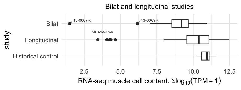
Figure 3.2: Boxplot displaying the muscle scores distribution of the bilateral, longitudinal and historical control samples. The dots present the outliers of low muscle content samples.
3.2 Characteristics of muscle-low samples
In Figure 3.2 and 3.1, we pinpoint the low muscle content outliers within the longitudinal and bilateral cohorts. Figure below demonstrates that the muscle-low outliers exhibiting the distinctive features characterized by low-to-undetected DUX4 signature and stronger disease-specific signatures compared to other FSHD samples (labeled as control-like and Moderate+).
NOTE: Refer to Appendix B for FSHD biopsies classification (categorized by Control-like and Moderate+) by the supervised machine learning algorithm.
load(file.path(pkg_dir, "data", "comprehensive_df.rda"))
pal <- wes_palette("Darjeeling1", n = 5)
names(pal) <- c('DUX4', 'ECM', 'Inflamm', 'IG', 'Complement')
comprehensive_df %>%
  dplyr::filter(!is.na(class)) %>%
  group_by(class) %>%
  summarise(DUX4 = mean(`DUX4-M6-logSum`),
            ECM = mean(`ECM-logSum`),
            Inflamm = mean(`Inflamm-logSum`),
            IG = mean(`IG-logSum`),
            Complement = mean(`Complement-logSum`)) %>%
  tidyr::gather(signature, average, -class) %>%
  dplyr::mutate(signature = factor(signature,
                                   levels=c('ECM', 'Inflamm', 'IG',
                                            'Complement', 'DUX4'))) %>%
  ggplot(aes(x=class, y=average, fill=signature)) +
    geom_bar(position="stack", stat="identity") +
    theme_light() +
    labs(title="Bilat cohort", y="Average signature score",
         x = "Categories") +
    scale_fill_manual(values= pal) +
    theme(panel.grid.minor = element_blank(),
          panel.grid.major = element_blank(),
          axis.text.x = element_text(angle = 90, vjust = 0.5, hjust=1))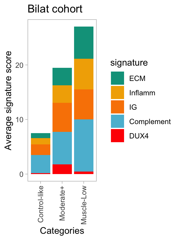
Figure 3.3: Average FSHD-disease signature scores across individual classes.
3.3 PCA and outlier confirmation
PCA reveals that biopsies exhibiting low muscle content, 13-0009R and 13-0007R, form a distinct cluster and are separated from the rest of the samples. Note that the class refers to the classification carried out by the supervise machine learning model, as detailed in Appendix B.
library(ggrepel)
load(file.path(pkg_dir, "data", "bilat_rlog.rda"))

data <- plotPCA(bilat_rlog, intgroup=c("class", "sample_id"), returnData=TRUE)
percentVar <- round(100 * attr(data, "percentVar"))
ggplot(data, aes(PC1, PC2, color=class)) +
  geom_point(size=2.5, alpha=0.8) +
  xlab(paste0("PC1: ",percentVar[1],"% variance")) +
  ylab(paste0("PC2: ",percentVar[2],"% variance")) +
  geom_text_repel(aes(label=sample_id), size=3,
                  show.legend=FALSE) +
  theme_minimal() +
  theme(legend.position="top",
        panel.grid.minor = element_blank())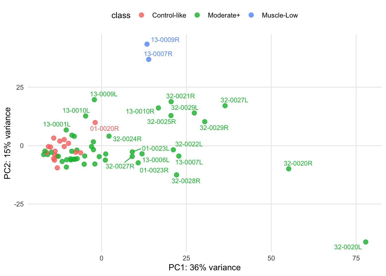
Figure 3.4: Biolat: PCA of regularized log transformation of the gene counts.