Create a data.frame to plot step lines — create_step

Creates survival probabilities from time and censoring information and generates a risk table that includes the survival probabilities and number at risk in addition to the data provided. This data.frame can be used to plot step line outcomes such as time-to-event (Kaplan-Meier curves) and magnitude breadth (MB) curves.

Usage

create_step_curve(x, event = NULL, flip_surv = FALSE, flip_top_x = Inf)

Arguments

x: Time values used to create the x-axis in step curves (numeric vector)
event: event status, 0=censor and 1=event (numeric vector). If NULL assumes no censoring
flip_surv: logical indicating if reverse survival estimates should be calculated. Default is FALSE.
flip_top_x: value to set x for top point for plotting. Only used if flip_surv = TRUE. Default is Inf.

Value

Returns a data frame with time, surv, n.risk, n.event, and n.censor (survival::summary.survfit output format). If flip_surv = TRUE also includes surv.flipped column.

Details

The output of survival probabilities can be used for plotting step function curves, with time on the x axis, surv on the y axis, and n.censor == 1 subset can be used for a ggplot2::geom_point() layer.

If flip_surv = TRUE there is an additional row at the bottom of the data.frame needed for horizontal line at the top of the plot

Examples


create_step_curve(x = 1:10)
#>    time surv n.risk n.event n.censor
#> 1     0  1.0     10      NA       NA
#> 2     1  0.9     10       1        0
#> 3     2  0.8      9       1        0
#> 4     3  0.7      8       1        0
#> 5     4  0.6      7       1        0
#> 6     5  0.5      6       1        0
#> 7     6  0.4      5       1        0
#> 8     7  0.3      4       1        0
#> 9     8  0.2      3       1        0
#> 10    9  0.1      2       1        0
#> 11   10  0.0      1       1        0
create_step_curve(x = 1:10, event = rep(0:1, 5))
#>    time      surv n.risk n.event n.censor
#> 1     0 1.0000000     10      NA       NA
#> 2     1 1.0000000     10       0        1
#> 3     2 0.8888889      9       1        0
#> 4     3 0.8888889      8       0        1
#> 5     4 0.7619048      7       1        0
#> 6     5 0.7619048      6       0        1
#> 7     6 0.6095238      5       1        0
#> 8     7 0.6095238      4       0        1
#> 9     8 0.4063492      3       1        0
#> 10    9 0.4063492      2       0        1
#> 11   10 0.0000000      1       1        0

library(dplyr)
dat = data.frame(x = c(1:10),
                 event = c(1,1,0,1,1,0,0,1,1,1),
                 ptid = c(1,1,2,2,3,3,3,3,3,3))
plot_data <-
 dat |>
  dplyr::group_by(ptid) |>
  dplyr::group_modify(~ create_step_curve(x = .x$x, event = .x$event))

ggplot2::ggplot(data = plot_data,
                ggplot2::aes(x = time, y = surv, color = factor(ptid))) +
 ggplot2::geom_step(linetype = "dashed", direction = 'hv', lwd = .35) +
 ggplot2::geom_point(data = plot_data |> filter(n.censor == 1),
                     shape = 3, size = 6, show.legend = FALSE)


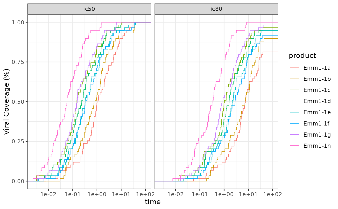
#mAB example for reverse curves
data(CAVD812_mAB)

plot_data <-
CAVD812_mAB |>
  filter(virus != 'SVA-MLV') |>
  tidyr::pivot_longer(cols = c(ic50, ic80)) |>
  dplyr::group_by(name, product) |>
  dplyr::group_modify(~ create_step_curve(x = pmin(.x$value, 100),
                                          event = as.numeric(.x$value < 50),
                                          flip_surv = TRUE,
                                          flip_top_x = 100))

ggplot2::ggplot(data = plot_data,
                ggplot2::aes(x = time, y = surv.flipped, color = product)) +
  ggplot2::geom_step(direction = 'hv', lwd = .35) +
  ggplot2::scale_x_log10() +
  ggplot2::scale_y_continuous('Viral Coverage (%)') +
  ggplot2::facet_grid(. ~ name) +
  ggplot2::theme_bw()
#> Warning: log-10 transformation introduced infinite values.