Overview and Introduction to VISCfunctions Package

Overview

VISCfunctions is a collection of useful functions designed to assist in the analysis and creation of professional reports. The current VISCfunctions package can be broken down to the following sections:

Testing and Estimate Functions
- two_samp_bin_test
- two_samp_cont_test
- cor_test
- binom_ci
- trapz_sorted
Fancy Output Functions
- pretty_pvalues
- stat_paste
- paste_tbl_grp
- escape
- collapse_group_row
Pairwise Comparison Functions
- pairwise_test_bin
- pairwise_test_cont
- cor_test_pairs
Survival and Magnitude Breadth
- create_step_curve
- mb_results
Utility Functions
- round_away_0
- get_session_info
- get_full_name
Example Datasets
- exampleData_BAMA
- exampleData_NAb
- exampleData_ICS
- CAVD812_mAB

Getting Started

Code to initially install the VISCfunctions package:


# Installing VISCfunctions from GitHub
remotes::install_github("FredHutch/VISCfunctions")

Code to load in VISCfunctions and start using:


# Loading VISCfunctions
library(VISCfunctions)

# Loading dplyr for pipe
library(dplyr)

VISCtemplates Package

The VISCtemplates package makes extensive use of the VISCfunctions package, and is a great way get started making professional statistical reports.

Code to initially download VISCtemplates package:


# Installing VISCfunctions from GitHub
remotes::install_github("FredHutch/VISCtemplates")

Once installed, in RStudio go to File -> New File -> R Markdown -> From Template -> VISC PT Report (Generic) to start a new Markdown report using the template. Within the template there is code to load and make use of most of the VISCfunctions functionality.

Example Datasets

The exampleData_BAMA, exampleData_NAb, exampleData_ICS, and CAVD812_mAB datasets are assay example datasets used throughout this vignette and most examples in the VISCfunctions documentation. All example datasets have associated documentation that can be viewed using ? (i.e ?exampleData_BAMA).


# Loading in example datasets
data("exampleData_BAMA", "exampleData_NAb", "exampleData_ICS", "CAVD812_mAB")

# Quick view of dataset
str(exampleData_BAMA)
#> 'data.frame':    252 obs. of  6 variables:
#>  $ pubID    : chr  "2435" "2435" "2435" "2435" ...
#>  $ group    : int  1 1 1 1 1 1 1 1 1 1 ...
#>  $ visitno  : num  0 0 0 0 0 0 0 1 1 1 ...
#>  $ antigen  : chr  "A1.con.env03 140 CF" "A244 D11gp120_avi" "B.63521_D11gp120/293F" "B.MN V3 gp70" ...
#>  $ magnitude: num  12 40.5 35.75 26.25 1.25 ...
#>  $ response : int  NA NA NA NA NA NA NA 1 1 1 ...

Testing and Estimate Functions

There are currently three testing functions performing the appropriate statistical tests, depending on the data and options, returning a p value.

There is also an estimate function for getting binary confidence intervals (binom_ci()).

trapz_sorted() is used to create an estimate for the area under a curve while making sure the x-axis is sorted so that both the x-axis and the area are increasing and positive, respectively.


# Making Testing Dataset
testing_data <- exampleData_BAMA |>
  dplyr::filter(antigen == 'A1.con.env03 140 CF' & visitno == 1)

Comparing Two Groups (Binary Variable) for a Binary Variable

two_samp_bin_test() is used for comparing a binary variable to a binary (two group) variable, with options for Barnard, Fisher’s Exact, Chi-Sq, and McNemar tests. For the Barnard test specifically, there are many model options that can be set that get passed to the Exact::exact.test() function.


table(testing_data$response, testing_data$group)
#>    
#>     1 2
#>   0 2 0
#>   1 4 6

# Barnard Method
two_samp_bin_test(
  x = testing_data$response,
  y = testing_data$group,
  method = 'barnard',
  alternative = 'two.sided'
)
#> [1] 0.1970196

# Santner and Snell Variation
two_samp_bin_test(
  x = testing_data$response,
  y = testing_data$group,
  method = 'barnard',
  barnard_method = 'santner and snell',
  alternative = 'two.sided')
#> [1] 0.3876953

# Calling test multiple times
exampleData_BAMA |> 
  group_by(antigen, visitno) |> 
  filter(visitno != 0) |> 
  summarise(p_val = two_samp_bin_test(response, group, method = 'barnard'), .groups = "drop")
#> # A tibble: 14 × 3
#>    antigen               visitno p_val
#>    <chr>                   <dbl> <dbl>
#>  1 A1.con.env03 140 CF         1 0.197
#>  2 A1.con.env03 140 CF         2 1    
#>  3 A244 D11gp120 avi           1 1    
#>  4 A244 D11gp120 avi           2 1    
#>  5 B.63521 D11gp120/293F       1 0.518
#>  6 B.63521 D11gp120/293F       2 1    
#>  7 B.MN V3 gp70                1 0.197
#>  8 B.MN V3 gp70                2 1    
#>  9 B.con.env03 140 CF          1 1    
#> 10 B.con.env03 140 CF          2 1    
#> 11 gp41                        1 0.667
#> 12 gp41                        2 0.774
#> 13 p24                         1 1    
#> 14 p24                         2 0.197

Comparing Two Groups (Binary Variable) for a Continuous Variable

two_samp_cont_test() is used for comparing a continuous variable to a binary (two group) variable, with parametric (t.test) and non-parametric (Wilcox Rank-Sum) options. Also paired data is allowed, where there are parametric (paired t.test) and non-parametric (Wilcox Signed-Rank) options.


by(testing_data$magnitude, testing_data$group, summary)
#> testing_data$group: 1
#>    Min. 1st Qu.  Median    Mean 3rd Qu.    Max. 
#>    9.75  253.44  648.00 1038.58 1321.00 3258.50 
#> ------------------------------------------------------------ 
#> testing_data$group: 2
#>    Min. 1st Qu.  Median    Mean 3rd Qu.    Max. 
#>   171.0   259.9   529.8   550.9   781.1  1040.2

two_samp_cont_test(
  x = testing_data$magnitude,
  y = testing_data$group,
  method = 'wilcox',
  alternative = 'two.sided'
)
#> [1] 0.6991342

# Calling test multiple times
exampleData_BAMA |> 
  group_by(antigen, visitno) |> 
  filter(visitno != 0) |> 
  summarise(p_val = two_samp_cont_test(magnitude, group, method = 'wilcox'), .groups = "drop")
#> # A tibble: 14 × 3
#>    antigen               visitno p_val
#>    <chr>                   <dbl> <dbl>
#>  1 A1.con.env03 140 CF         1 0.699
#>  2 A1.con.env03 140 CF         2 0.589
#>  3 A244 D11gp120 avi           1 0.699
#>  4 A244 D11gp120 avi           2 0.394
#>  5 B.63521 D11gp120/293F       1 0.937
#>  6 B.63521 D11gp120/293F       2 0.937
#>  7 B.MN V3 gp70                1 0.699
#>  8 B.MN V3 gp70                2 0.180
#>  9 B.con.env03 140 CF          1 0.699
#> 10 B.con.env03 140 CF          2 0.589
#> 11 gp41                        1 0.310
#> 12 gp41                        2 0.485
#> 13 p24                         1 0.485
#> 14 p24                         2 0.240

Comparing Two Continuous Variables (Correlation)

cor_test() is used for comparing two continuous variables, with Pearson, Kendall, or Spearman methods.

If Spearman method is chosen and either variable has a tie, the approximate distribution is use in the coin::spreaman_test() function. This is usually the preferred method over the asymptotic approximation, which is the method stats:cor.test() uses in cases of ties. If the Spearman method is chosen and there are no ties, the exact method is used from stats:cor.test.


# Making Testing Dataset
cor_testing_data <- exampleData_BAMA |>
  dplyr::filter(antigen %in% c('A1.con.env03 140 CF', 'B.MN V3 gp70'),
                visitno == 1,
                group == 1) |>
  tidyr::pivot_wider(id_cols = pubID,
                     names_from = antigen,
                     values_from = magnitude)

stats::cor(cor_testing_data$`A1.con.env03 140 CF`,
           cor_testing_data$`B.MN V3 gp70`,
           method = 'spearman')
#> [1] -0.4285714

cor_test(
  x = cor_testing_data$`A1.con.env03 140 CF`,
  y = cor_testing_data$`B.MN V3 gp70`,
  method = 'spearman'
)
#> [1] 0.4194444

Computing the Area Under a Curve (Integration Estimate) for Messy Data

trapz_sorted() is used when you are not presorting your data so that it is strictly increasing along the x-axis or when there are ‘NA’ values that are not removed prior to estimating the area under the curve.

set.seed(93)
n <- 10
# unsorted data
x <- sample(1:n, n, replace = FALSE)
y <- runif(n, 0, 42)
pracma::trapz(x, y)
#> [1] 97.44204
trapz_sorted(x,y)
#> [1] 213.7732

# NA in data
x <- c(1:6, NA, 8:10)
y[2] <- NA
pracma::trapz(x, y)
#> [1] NA
trapz_sorted(x,y, na.rm = TRUE)
#> [1] 208.5765

Fancy Output Functions

These are functions designed to produce professional output that can easily be printed in reports.

P Values

pretty_pvalues() is used on p-values by rounding them to a specified number of digits and using < for low p-values as opposed to scientific notation (i.e., “p < 0.0001” if rounding to 4 digits), and by allowing options for emphasizing p-values and specific characters for missing values.


pvalue_example = c(1, 0.06753, 0.004435, NA, 1e-16, 0.563533)
# For simple p value display
pretty_pvalues(pvalue_example, digits = 3, output_type = 'no_markup')
#> [1] "1.000"  "0.068"  "0.004"  "---"    "<0.001" "0.564"

# For display in report
table_p_Values <- pretty_pvalues(pvalue_example, digits = 3, 
                                 background = "yellow")
kableExtra::kable(
  table_p_Values,
  escape = FALSE,
  linesep = "",
  col.names = c("P-values"),
  caption = 'Fancy P Values'
) |>
  kableExtra::kable_styling(font_size = 8.5,
                            latex_options = "hold_position")

You can also specify if you want p= pasted on the front of the p values, using the include_p parameter.

Basic Combining of Variables

stat_paste() is used to combine two or three statistics together, allowing for different rounding and bound character specifications. Common uses for this function are for:

Mean (sd)
Median [min, max]
Estimate (SE of Estimate)
Estimate (95% CI Lower Bound, Upper Bound)
Estimate/Statistic (p value)

# Simple Examples
stat_paste(stat1 = 2.45, stat2 = 0.214, stat3 = 55.3, 
           digits = 2, bound_char = '[')
#> [1] "2.45 [0.21, 55.30]"
stat_paste(stat1 = 6.4864, stat2 = pretty_pvalues(0.0004, digits = 3), 
           digits = 3, bound_char = '(')
#> [1] "6.486 (<0.001)"

exampleData_BAMA |> 
  filter(visitno == 1) |>  
  group_by(antigen, group) |> 
  reframe(`Magnitude Info (Median [Range])` = 
            stat_paste(stat1 = median(magnitude), 
                       stat2 = min(magnitude),
                       stat3 = max(magnitude),
                       digits = 2, bound_char = '['),
          `Magnitude Info (Mean (SD))` = 
            stat_paste(stat1 = mean(magnitude), 
                       stat2 = sd(magnitude),
                       digits = 2, bound_char = '('))
#> # A tibble: 14 × 4
#>    antigen               group Magnitude Info (Median […¹ Magnitude Info (Mean…²
#>    <chr>                 <int> <chr>                      <chr>                 
#>  1 A1.con.env03 140 CF       1 648.00 [9.75, 3258.50]     1038.58 (1210.00)     
#>  2 A1.con.env03 140 CF       2 529.75 [171.00, 1040.25]   550.92 (347.74)       
#>  3 A244 D11gp120 avi         1 2542.88 [166.25, 19183.25] 5655.17 (7413.17)     
#>  4 A244 D11gp120 avi         2 1046.12 [430.00, 3704.00]  1680.71 (1348.20)     
#>  5 B.63521 D11gp120/293F     1 1562.88 [69.50, 3910.50]   1719.88 (1572.96)     
#>  6 B.63521 D11gp120/293F     2 675.88 [307.75, 5115.50]   1577.17 (1894.48)     
#>  7 B.MN V3 gp70              1 117.38 [-36.25, 329.00]    140.04 (158.30)       
#>  8 B.MN V3 gp70              2 14.13 [-618.75, 2425.00]   302.71 (1105.90)      
#>  9 B.con.env03 140 CF        1 2819.25 [191.25, 5989.75]  3149.50 (2364.75)     
#> 10 B.con.env03 140 CF        2 4897.62 [589.75, 13738.25] 5152.88 (4685.93)     
#> 11 gp41                      1 14377.75 [5380.75, 26021.… 16323.67 (8023.22)    
#> 12 gp41                      2 25038.50 [8504.50, 32447.… 22558.67 (10658.01)   
#> 13 p24                       1 6688.12 [1728.00, 13559.0… 6745.00 (4760.00)     
#> 14 p24                       2 3265.50 [963.50, 9886.25]  3880.46 (3180.21)     
#> # ℹ abbreviated names: ¹`Magnitude Info (Median [Range])`,
#> #   ²`Magnitude Info (Mean (SD))`

Advanced Combining of Variables

paste_tbl_grp() pastes together information, often statistics, from two groups. There are two predefined combinations: mean(sd) and median[min,max], but user may also paste any single measure together.

Example of summary information to be pasted together (partial output):

#> # A tibble: 7 × 6
#>   antigen               Group1_max Group1_mean Group1_median Group1_min Group1_n
#>   <chr>                      <dbl>       <dbl>         <dbl>      <dbl>    <dbl>
#> 1 A1.con.env03 140 CF        3258.       1039.          648        9.75        6
#> 2 A244 D11gp120 avi         19183.       5655.         2543.     166.          6
#> 3 B.63521 D11gp120/293F      3910.       1720.         1563.      69.5         6
#> 4 B.MN V3 gp70                329         140.          117.     -36.2         6
#> 5 B.con.env03 140 CF         5990.       3150.         2819.     191.          6
#> 6 gp41                      26022.      16324.        14378.    5381.          6
#> 7 p24                       13559        6745          6688.    1728           6


summary_table <-  summary_info |>
  paste_tbl_grp(
    vars_to_paste = c('n', 'mean_sd', 'median_min_max'),
    first_name = 'Group1',
    second_name = 'Group2'
  )

kableExtra::kable(
  summary_table,
  booktabs = TRUE,
  linesep = "",
  caption = 'Summary Information Comparison'
) |>
  kableExtra::kable_styling(font_size = 6.5, latex_options = "hold_position") |>
  kableExtra::footnote('Summary Information for Group 1 vs. Group 2, by Antigen and for Visit 1')

Escape

escape() protects control characters in a string for use in a latex table or caption.


value_example <- c("testvalue", "test_value", "ampersand&")
escape(value_example)
#> [1] "testvalue"    "test\\_value" "ampersand\\&"
escape("String_Entry %")
#> [1] "String\\_Entry \\%"

Collapsing Rows

collapse_group_row() is for replacing repeated rows in a data.frame into NA for nice printing. This is an alternative to kableExtra::collapse_rows(), which does not work well for tables that span multiple pages (i.e. longtable = TRUE).

set.seed(341235432)
sample_df <- data.frame(
  x = c(1, 1, 1, 2, 2, 2, 2),
  y = c('test1', 'test1', 'test2', 'test1', 'test2', 'test2', 'test1'),
  z = c(1, 2, 3, 4, 5, 6, 7),
  outputVal = runif(7)
)

collapse_group_row(sample_df, x, y, z) |>
  kableExtra::kable(
    booktabs = TRUE,
    linesep = "",
    row.names = FALSE
  ) |>
  kableExtra::row_spec(3, hline_after = TRUE) |> 
  kableExtra::kable_styling(font_size = 8, latex_options = "hold_position")

Pairwise Comparison Functions

pairwise_test_bin(), pairwise_test_cont(), cor_test_pairs() are functions that perform pairwise group (or any categorical variable) comparisons. The function will go through all pairwise comparisons and output descriptive statistics and relevant p values, calling the appropriate testing functions from the Testing and Estimate Functions section.

Pairwise Comparison of Multiple Groups for a Binary Variable

Simple example using pairwise_test_bin:


set.seed(1)
x_example <- c(NA, sample(0:1, 50, replace = TRUE, prob = c(.75, .25)),
  sample(0:1, 50, replace = TRUE, prob = c(.25, .75)))
group_example <- c(rep(1, 25), NA, rep(2, 25), rep(3, 25), rep(4, 25))

pairwise_test_bin(x_example, group_example) |> 
  rename(Separation = 'PerfectSeparation')
#>   Comparison                                                 ResponseStats
#> 1    1 vs. 2   7/24 = 29.2% (14.9%, 49.2%) vs. 6/25 = 24.0% (11.5%, 43.4%)
#> 2    1 vs. 3  7/24 = 29.2% (14.9%, 49.2%) vs. 20/25 = 80.0% (60.9%, 91.1%)
#> 3    1 vs. 4  7/24 = 29.2% (14.9%, 49.2%) vs. 16/25 = 64.0% (44.5%, 79.8%)
#> 4    2 vs. 3  6/25 = 24.0% (11.5%, 43.4%) vs. 20/25 = 80.0% (60.9%, 91.1%)
#> 5    2 vs. 4  6/25 = 24.0% (11.5%, 43.4%) vs. 16/25 = 64.0% (44.5%, 79.8%)
#> 6    3 vs. 4 20/25 = 80.0% (60.9%, 91.1%) vs. 16/25 = 64.0% (44.5%, 79.8%)
#>    ResponseTest Separation
#> 1 0.76819476151      FALSE
#> 2 0.00038580518      FALSE
#> 3 0.01666966048      FALSE
#> 4 0.00009064775      FALSE
#> 5 0.00498314375      FALSE
#> 6 0.23445322077      FALSE

Group comparison example using pairwise_test_bin:


## Group Comparison
group_testing <- exampleData_ICS |>
  filter(Population == 'IFNg Or IL2' & Group != 4) |>
  group_by(Stim, Visit) |>
  group_modify( ~ as.data.frame(
    pairwise_test_bin(x = .$response, group = .$Group,
                      method = 'barnard', alternative = 'less',
                      num_needed_for_test = 3, digits = 1,
                      latex_output = TRUE, verbose = FALSE
                      )
  )) |>
  ungroup() |>
  # Getting fancy p values
  mutate(
    ResponseTest = pretty_pvalues(
      ResponseTest, output_type = 'latex',
      sig_alpha = .1, background = 'yellow'
    )
  )


kableExtra::kable( group_testing, escape = FALSE, booktabs = TRUE,
  linesep = "", caption = 'Response Rate Comparisons Across Groups'
) |>
  kableExtra::kable_styling(
    font_size = 6.5,
    latex_options = c("hold_position", "scale_down")
    ) |>
  kableExtra::collapse_rows(c(1:2),
                            row_group_label_position = 'identity',
                            latex_hline = 'full')

Time point comparison example (paired) using pairwise_test_bin():


## Timepoint Comparison
timepoint_testing <- exampleData_ICS |>
  filter(Population == 'IFNg Or IL2' & Group != 4) |> 
  group_by(Stim, Group) |>
  group_modify(~ as.data.frame(
    pairwise_test_bin(x = .$response, group = .$Visit, id = .$pubID,
                      method = 'mcnemar', num_needed_for_test = 3, digits = 1,
                      latex_output = TRUE, verbose = FALSE))) |> 
  ungroup() |> 
  # Getting fancy p values
  mutate(ResponseTest = pretty_pvalues(ResponseTest, output_type = 'latex', 
                                       sig_alpha = .1, background = 'yellow'))


kableExtra::kable(timepoint_testing, escape = FALSE, booktabs = TRUE, 
                  caption = 'Response Rate Comparisons Across Visits') |> 
  kableExtra::kable_styling(font_size = 6.5, 
                            latex_options = c("hold_position","scale_down")) |> 
  kableExtra::collapse_rows(c(1:2), row_group_label_position = 'identity', 
                            latex_hline = 'full')

Pairwise Comparison of Multiple Groups for a Continuous Variable

Simple example using pairwise_test_cont():


set.seed(1)
x_example <- c(NA, rnorm(50), rnorm(50, mean = 5))
group_example <- c(rep(1, 25), rep(2, 25), rep(3, 25), rep(4, 25), NA)

pairwise_test_cont(x_example, group_example, digits = 1) |> 
  rename(Separation = 'PerfectSeparation')
#>   Comparison SampleSizes                       Median_Min_Max
#> 1    1 vs. 2   24 vs. 25 0.4 [-2.2, 1.6] vs. -0.1 [-1.5, 1.4]
#> 2    1 vs. 3   24 vs. 25   0.4 [-2.2, 1.6] vs. 5.2 [0.9, 7.4]
#> 3    1 vs. 4   24 vs. 25   0.4 [-2.2, 1.6] vs. 5.1 [3.5, 6.6]
#> 4    2 vs. 3   25 vs. 25  -0.1 [-1.5, 1.4] vs. 5.2 [0.9, 7.4]
#> 5    2 vs. 4   25 vs. 25  -0.1 [-1.5, 1.4] vs. 5.1 [3.5, 6.6]
#> 6    3 vs. 4   25 vs. 25    5.2 [0.9, 7.4] vs. 5.1 [3.5, 6.6]
#>                   Mean_SD          MagnitudeTest Separation
#> 1 0.1 (1.0) vs. 0.0 (0.7) 0.28742747500751675283      FALSE
#> 2 0.1 (1.0) vs. 5.1 (1.4) 0.00000000000060121537      FALSE
#> 3 0.1 (1.0) vs. 5.0 (0.9) 0.00000000000003164291       TRUE
#> 4 0.0 (0.7) vs. 5.1 (1.4) 0.00000000000006328583      FALSE
#> 5 0.0 (0.7) vs. 5.0 (0.9) 0.00000000000001582146       TRUE
#> 6 5.1 (1.4) vs. 5.0 (0.9) 0.86260828521739307817      FALSE

Group comparison example using pairwise_test_cont():


## Group Comparison
group_testing <- exampleData_ICS |>
  filter(Population == 'IFNg Or IL2' & Group != 4) |> 
  group_by(Stim, Visit) |>
  group_modify(~ as.data.frame(
    pairwise_test_cont(x = pmax(.$PercentCellNet, 0.00001), group = .$Group,
                      method = 'wilcox', paired = FALSE, 
                      alternative = 'greater', num_needed_for_test = 3, 
                      digits = 3, log10_stats = TRUE))) |> 
   ungroup() |> 
  # Getting fancy p values
  mutate(MagnitudeTest = pretty_pvalues(
    MagnitudeTest, output_type = 'latex', 
    sig_alpha = .1, background = 'yellow')
  ) |> 
  rename("Median (Range)" = Median_Min_Max, 'Mean (SD) (log10)' = log_Mean_SD)

kableExtra::kable(group_testing, escape = FALSE, booktabs = TRUE, 
                  caption = 'Magnitude Comparisons Across Groups') |> 
  kableExtra::kable_styling(font_size = 6.5, 
                            latex_options = c("hold_position","scale_down")) |> 
  kableExtra::collapse_rows(c(1:2), 
                            row_group_label_position = 'identity', 
                            latex_hline = 'full')

Time point comparison example (paired) using pairwise_test_cont():


## Timepoint Comparison
timepoint_testing <- exampleData_ICS |>
  filter(Population == 'IFNg Or IL2' & Group != 4) |> 
  group_by(Stim, Group) |>
  group_modify(~ as.data.frame(
    pairwise_test_cont(x =  pmax(.$PercentCellNet, 0.00001), group = .$Visit, 
                       id = .$pubID, method = 'wilcox', paired = TRUE, 
                       num_needed_for_test = 3, 
                       digits = 3, log10_stats = TRUE))) |> 
   ungroup() |> 
  # Getting fancy p values
  mutate(MagnitudeTest = pretty_pvalues(
    MagnitudeTest, output_type = 'latex', 
    sig_alpha = .1, background = 'yellow')
    ) |> 
  rename("Median (Range)" = Median_Min_Max, 'Mean (SD) (log10)' = log_Mean_SD)


kableExtra::kable(timepoint_testing, 
                  escape = FALSE, 
                  booktabs = TRUE, 
                  caption = 'Magnitude Comparisons Across Visits') |> 
  kableExtra::kable_styling(font_size = 6.5, 
                            latex_options = c("hold_position","scale_down")) |> 
  kableExtra::collapse_rows(c(1:2), 
                            row_group_label_position = 'identity', 
                            latex_hline = 'full')

Pairwise Comparison of Continuous Variables (Correlation)

Simple example using cor_test_pairs:


set.seed(1)
x_example <- c(1, 1, rnorm(48), rnorm(49, mean = 5), NA)
pair_example <- c(rep('antigen A', 25), rep('antigen B', 25), 
                   rep('antigen C', 25), rep('antigen D', 25))
id_example <- c(rep(1:25, 4))

cor_test_pairs(x_example, pair_example, id_example, digits = 4)
#>               Correlation NPoints              Ties CorrEst  CorrTest
#> 1 antigen A and antigen B      25 ties in antigen A -0.1012 0.6263000
#> 2 antigen A and antigen C      25 ties in antigen A -0.0727 0.7186000
#> 3 antigen A and antigen D      24 ties in antigen A  0.0100 0.9666000
#> 4 antigen B and antigen C      25           no ties  0.1754 0.3999939
#> 5 antigen B and antigen D      24           no ties -0.1530 0.4735370
#> 6 antigen C and antigen D      24           no ties -0.1087 0.6118973

Correlation comparisons using cor_test_pairs:

## Antigen Correlations
antigen_testing <- exampleData_BAMA |>
  filter(antigen %in% c('B.63521 D11gp120/293F', 
                        'B.con.env03 140 CF',
                        'B.MN V3 gp70') & 
           group != 4) |> 
  group_by(group, visitno) |>
  group_modify(~ as.data.frame(
    cor_test_pairs(x = .x$magnitude,
                      pair = .x$antigen,
                      id = .x$pubID,
                      method = 'spearman',
                      n_distinct_value = 3))) |> 
  ungroup() |> 
  # Getting fancy p values
  mutate(CorrTest = pretty_pvalues(CorrTest, output_type = 'latex', 
                                   sig_alpha = .1, background = 'yellow')) |> 
  rename("Corr P Value" = CorrTest)

kableExtra::kable(antigen_testing, escape = FALSE, 
                  booktabs = TRUE, caption = 'Correlations between Antigen') |> 
  kableExtra::kable_styling(font_size = 6.5, 
                            latex_options = c("hold_position","scale_down")) |> 
  kableExtra::collapse_rows(c(1:2), 
                            row_group_label_position = 'identity', 
                            latex_hline = 'full')

Survival and Magnitude Breadth

create_step_curve() creates survival probabilities from time and censoring information and generates a risk table that includes the survival probabilities and number at risk in addition to the data provided. This output can be used to plot step line outcomes such as time-to-event (Kaplan-Meier curves), magnitude breadth (MB) curves, and cumulative plots.


#Potency-breadth curves
plot_data <-
 CAVD812_mAB |>
  filter(virus != 'SVA-MLV') |> 
  tidyr::pivot_longer(cols = c(ic50, ic80)) |> 
  dplyr::group_by(name, product) |>
  dplyr::group_modify(~ create_step_curve(x = pmin(.x$value, 100), 
                                          event = as.numeric(.x$value < 50),
                                          flip_surv = TRUE, flip_top_x = 100)) 
  
  ggplot2::ggplot(data = plot_data,
                  ggplot2::aes(x = time, y = 1 - surv, color = product)) +
  ggplot2::geom_step(direction = 'hv', lwd = .35) +
  ggplot2::scale_x_log10() +
  ggplot2::scale_y_continuous('Viral Coverage (%)') +
  ggplot2::facet_grid(. ~ name) +
  ggplot2::theme_bw()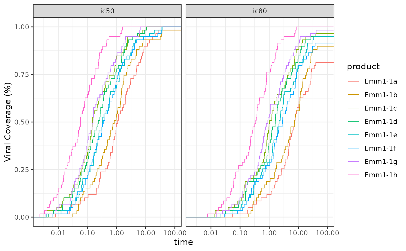

Potency-breath curves

mb_results() creates step curve info for magnitude breadth (MB) plots, with options to include response status and have logged transformation for AUC-MB calculation.

data_here <- exampleData_BAMA |> filter(visitno == 2)

group_results <- data_here |> dplyr::group_by(group) |>
  dplyr::group_modify(~ mb_results(magnitude = .x$magnitude , 
                                   response = .x$response))
ind_results <-  data_here |> dplyr::group_by(group, pubID) |>
  dplyr::group_modify(~ mb_results(magnitude = .x$magnitude , 
                                   response = .x$response))
ggplot2::ggplot(
  data = group_results,
  ggplot2::aes(x = magnitude, y = breadth, color = factor(group))) +
  ggplot2::geom_step(data = ind_results, ggplot2::aes(group = pubID),
                     linetype = "dashed", direction = 'hv', lwd = .35, alpha = .7) +
  ggplot2::geom_step(direction = 'hv', lwd = .65) +
  ggplot2::scale_x_log10('Response Magnitude',
    breaks = c(100,1000,10000, 22000),
    labels = c(expression("" <= 100),1000,10000, expression("" >= 22000))) +
  ggplot2::ylab('Magnitude Breadth (%)') +
  ggplot2::scale_color_discrete('Group') +
  ggplot2::coord_cartesian(xlim = c(95, 23000)) +
  ggplot2::theme_bw()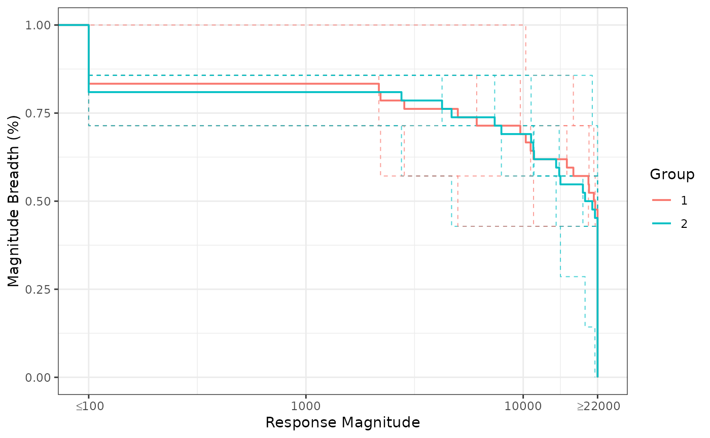

BAMA Magnitude Breadth curves


# AUC-MB plot
AUC_MB <- dplyr::distinct(ind_results, group, pubID, aucMB)

ggplot2::ggplot(AUC_MB, ggplot2::aes(x = factor(group), y = aucMB,
                                     color = factor(group))) +
  ggplot2::geom_boxplot(outlier.color = NA, show.legend = FALSE) +
  ggplot2::geom_point(position = ggplot2::position_jitter(width = 0.25,
           height = 0, seed = 1), size = 1.5, show.legend = FALSE) +
  ggplot2::scale_y_log10('AUC-MB') +
  ggplot2::xlab('Group') +
  ggplot2::theme_bw()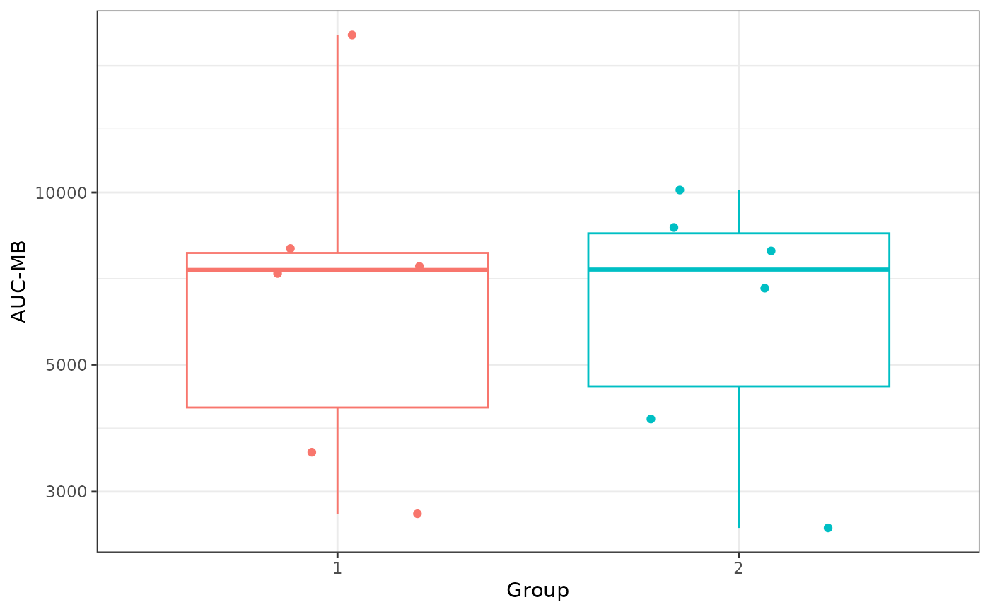

BAMA Magnitude Breadth curves

Utility Functions

round_away_0() is a function to properly perform mathematical rounding (i.e. rounding away from 0 when tied), as opposed to the round() function, which rounds to the nearest even number when tied. Also round_away_0() allows for trailing zeros (i.e. 0.100 if rounding to 3 digits).

vals_to_round = c(NA,-3.5:3.5)
vals_to_round
#> [1]   NA -3.5 -2.5 -1.5 -0.5  0.5  1.5  2.5  3.5
round(vals_to_round)
#> [1] NA -4 -2 -2  0  0  2  2  4
round_away_0(vals_to_round)
#> [1] NA -4 -3 -2 -1  1  2  3  4
round_away_0(vals_to_round, digits = 2, trailing_zeros = TRUE)
#> [1] NA      "-3.50" "-2.50" "-1.50" "-0.50" "0.50"  "1.50"  "2.50"  "3.50"

get_session_info() produces reproducible tables, which are great to add to the end of reports. The first table gives software session information and the second table gives software package version information. get_full_name() is a function used by get_session_info() to get the user’s name, based on user’s ID.

my_session_info <- get_session_info()
kableExtra::kable(
  my_session_info$platform_table,
  booktabs = TRUE,
  linesep = '',
  caption = "Reproducibility Software Session Information"
) |>
  kableExtra::kable_styling(font_size = 8, latex_options = "hold_position")


kableExtra::kable(
  my_session_info$packages_table,
  booktabs = TRUE,
  linesep = '',
  caption = "Reproducibility Software Package Version Information"
) |>
  kableExtra::kable_styling(font_size = 8, latex_options = "hold_position")

Jimmy Fulp, Monica Gerber, and Heather Bouzek

2026-01-16

Overview

Getting Started

VISCtemplates Package

Example Datasets

Testing and Estimate Functions

Comparing Two Groups (Binary Variable) for a Binary Variable

Comparing Two Groups (Binary Variable) for a Continuous Variable

Comparing Two Continuous Variables (Correlation)

Computing the Area Under a Curve (Integration Estimate) for Messy Data

Fancy Output Functions

P Values

Basic Combining of Variables

Advanced Combining of Variables

Escape

Collapsing Rows

Pairwise Comparison Functions

Pairwise Comparison of Multiple Groups for a Binary Variable

Pairwise Comparison of Multiple Groups for a Continuous Variable

Pairwise Comparison of Continuous Variables (Correlation)

Survival and Magnitude Breadth

Utility Functions