Chapter 3 Follow-up visit

This chapter is dedicated to the one-year follow-up visit RNA-seq analysis and correlation to MRI characteristics and histopathology scores.

3.1 Loading datasets

First of all, we load the libraries and sanitized.dds, year2.dds, and mri_pathology datasets.

suppressPackageStartupMessages(library(DESeq2))
suppressPackageStartupMessages(library(xlsx))
suppressPackageStartupMessages(library(ggplot2))
suppressPackageStartupMessages(library(tidyverse))
suppressPackageStartupMessages(library(BiocParallel))
multi_param <- MulticoreParam(worker=2)
register(multi_param, default=TRUE)

pkg_dir <- "/fh/fast/tapscott_s/CompBio/RNA-Seq/hg38.FSHD.biopsy.all"

source(file.path(pkg_dir, "scripts", "manuscript_tools.R"))
load(file.path(pkg_dir, "public_data", "sanitized.dds.rda"))
load(file.path(pkg_dir, "public_data", "mri_pathology.rda"))
load(file.path(pkg_dir, "public_data", "year2.dds.rda"))

3.2 The follow-up visit RNA-seq dataset

The follow-up visit RNA-seq dataset, year2.dds, consists with 8 controls and 27 FSHD follow-up visit samples. It is a subset of sanitized.dds and the normalization excludes the initial visit. Chuck below shows the process of subsetting sanitized.dds and getting the normalization factor of the year2.dds instance.

keep_column_2 <- (sanitized.dds$visit == "II" | sanitized.dds$pheno_type == "Control") 
year2.dds <- sanitized.dds[, keep_column_2]
year2.dds$batch <- factor(year2.dds$batch)

#' re-normalized again, get the size factors and dispersion estimations
year2.dds <- estimateSizeFactors(year2.dds)
year2.dds <- estimateDispersions(year2.dds)
design(year2.dds) <- ~ pheno_type 
#year2.rlg <- rlog(year2.dds, blind = TRUE) #normalized with respect to year2 library size

3.3 DUX4 and other marker scores

The DUX4 score of RNA-seq biopsy samples is based on four FSHD/DUX4-positive biomarkers that were previously found in Yao 2014(Yao and al. 2014). Additional marker scores from other function category (extracellular matrix, immune/inflamm, cell cycle and immunoglobulin) are based on selected discriminative genes that shape the cluster pattern of the samples captured by Principal Components Analysis (top PC1/PC2 loading variables). The marker score is calculated as the sum of the these for biomarkers’ local regularized log Love 2014(Love, Huber, and Anders 2014) scaling difference from the control average. The code chunk below defines the markers for five different biological functions: $score=\sum_i^n g_i - \sum_i^n g_{i, control}$, where $g_i$ is the $i$th gene rlog expression in the function category and similary $g_{i, control} $ is the $i$th average gene expression in the function category from the controls.

#' define the determinative genes and calculate the marker scores
markers_list <- 
  list(dux4 = c("LEUTX", "KHDC1L", "PRAMEF2", "TRIM43"),
       extracellular_matrix = c("PLA2G2A", "COL19A1", "COMP", "COL1A1"), 
       inflamm = c("CCL18", "CCL13" ,"C6", "C7"), 
       cell_cycle = c("CCNA1", "CDKN1A", "CDKN2A"), 
       immunoglobulin = c("IGHA1", "IGHG4", "IGHGP")) 
#' get local rlog                            
markers_id_list <- lapply(markers_list, get_ensembl, rse=year2.dds)
relative_rlg <- lapply(markers_id_list, .get_sum_relative_local_rlg,
                       dds = year2.dds)

Table 3.1: Selected Genes used to calculate the marker scores.
	biomarkers/genes
dux4	LEUTX, KHDC1L, PRAMEF2, TRIM43
extracellular_matrix	PLA2G2A, COL19A1, COMP, COL1A1
inflamm	CCL18, CCL13, C6, C7
cell_cycle	CCNA1, CDKN1A, CDKN2A
immunoglobulin	IGHA1, IGHG4, IGHGP

Append the marker scores to year2.dds.

#' (1a) Append markers score to colData of year2.dds and year2.rlg
df <- as.data.frame(do.call(cbind, relative_rlg)) %>%
  dplyr::rename(dux4.rlogsum=dux4, ecm.rlogsum=extracellular_matrix, 
                inflamm.rlogsum=inflamm, cellcycle.rlogsum=cell_cycle,
                img.rlogsum=immunoglobulin)       

if (!any(names(colData(year2.dds)) %in% "dux4.rlogsum")) {
  colData(year2.dds) <- append(colData(year2.dds), 
                               as(df[colnames(year2.dds), ], "DataFrame"))
}

3.3.1 Group samples by DUX4 score

We divide the controls and the one-year follow-up FSHD samples into four sub-groups (G1-G4) based on their DUX4 scores and hierarchical clustering.

dux4_local_rlog <- .get_local_rlg(markers_id_list$dux4, year2.dds)
dux4_tree <- .get_DUX4_clust_tree(dux4_rlog=dux4_local_rlog)
year2.dds$dux4.group <- dux4_tree[colnames(year2.dds)]

3.3.2 Heatmap of the discriminative genes

Heatmap below presents the z-score (by rows) of local rlog expression of the selected, discriminative genes from different function categories. The DUX4 target genes displayed in the heatmap are not the main biomarkers for DUX4 score calculation, but instead are the genes (ZSCAN4, MBD3L2 and PRAMEF25) that also shows equivalent discriminative power in cluster pattern recognition.

library(pheatmap)
library(reshape2)
tmp <- markers_id_list
alt_dux4 <- get_ensembl(c("ZSCAN4", "MBD3L2", "PRAMEF25"), year2.dds)
tmp$dux4 <- alt_dux4
selected <- melt(tmp)
data <- as.matrix(.get_local_rlg(as.character(selected$value), year2.dds))
data <- data[as.character(selected$value), ]
rownames(data) <- rowData(year2.dds[rownames(data)])$gene_name
zscore_data <- (data - rowMeans(data)) / rowSds(data)

annotation_col <- data.frame(pheno_type=year2.dds$pheno_type,
                             dux4_group=factor(year2.dds$dux4.group))
rownames(annotation_col) <- colnames(year2.dds)
annotation_row <- data.frame(marker_type=selected$L1)
rownames(annotation_row) <- rownames(data)
row_gaps <- cumsum(sapply(tmp, length))

pheatmap(zscore_data, annotation_col=annotation_col, cellheight=8,
         fontsize_row = 7, fontsize = 7,
         cluster_rows = FALSE, gaps_row = row_gaps,
         annotation_row=annotation_row, scale="none")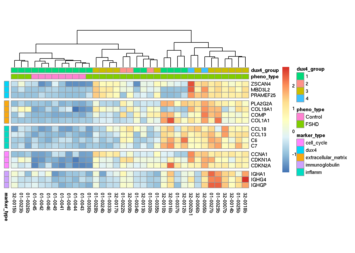

Figure 3.1: Heatmap of distcriminative genes from five function categories.

3.4 DUX4 candidate biomarkers are eleveated in FSHD

library(gridExtra)
file_name <- file.path(pkg_dir, "figures", "Year2_Scatter_FourBiomarkers.pdf")
gobj <- 
  .makeFourBiomarkerScatterPlot(dds=year2.dds, plot.tile_top=FALSE,
                                group=year2.dds$dux4.group,
                                markers_id=markers_id_list$dux4,
                                call_threshold=2,
                                file_name=file_name)

The scatter plot blow is Fig. 1 in the manuscript showing the relative expression of four candidate biomarkers in muscle biopsies from control and follow-up visit FSHD muscles. The sum of the relative expression of four DUX4-regulated genes (LEUTX, KHDC1L, TRIM43 and PRAMEF2) was plotted for each RNA-seq sample. The FSHD biopsies from follow-up visit are indicated by an asterisk (*), whereas control muscle biopsies do not have an asterisk. The size of the spot reflects the number of candidate biomarkers above a threshold level for considering elevated expression from the controls (log fold > 2).

grid.arrange(gobj$tilePlot, gobj$scatterPlot, nrow=2, ncol=1, heights=c(1,3))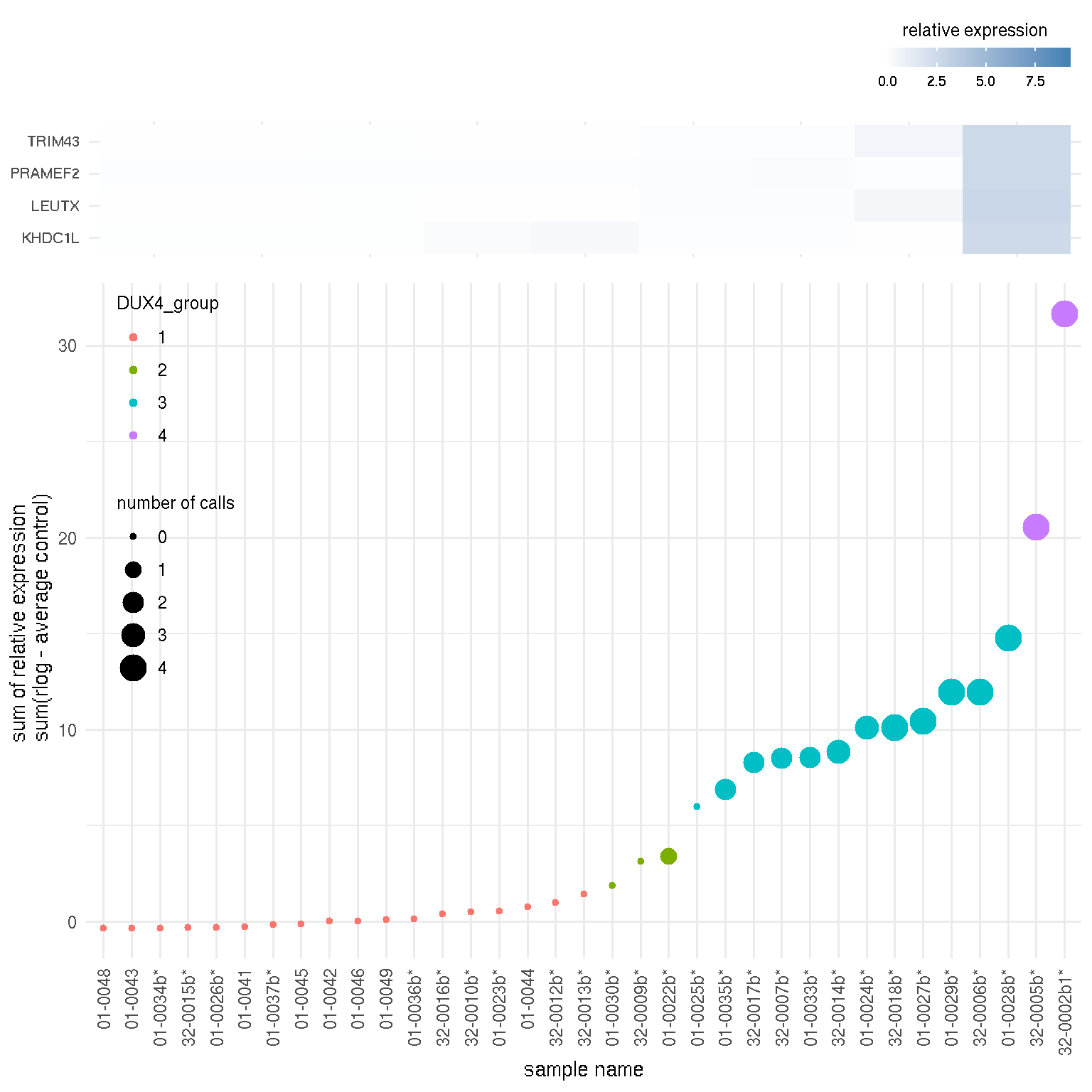

Figure 3.2: Scatter plot of DUX4 marker score by samples and sample groups by DUX4 score.

3.5 Correlation of DUX4 score to MRI and histopathology

DUX4 score is represented as the sum of relative rlog expression of four DUX4 biomarkers. Code chunk prepares a data.frame appending DUX4 scores to the histopathology scores and MRI signals.

dux4_score <- colData(year2.dds)[, c("sample_name", "dux4.rlogsum", "dux4.group")]
time_2 <- mri_pathology[["time_2"]] %>% 
  left_join(as.data.frame(dux4_score), by="sample_name") %>% 
  dplyr::filter(!is.na(Pathology.Score)) %>%
  rename(DUX4.Score = dux4.rlogsum)

3.5.1 DUX4 and pathology score

Similar to the first year, DUX4 score shows moderate correlation to pathology score (0.507).

cor <- cor(time_2$Pathology.Score, time_2$DUX4.Score,
           method="spearman")
ggplot(time_2, aes(x=Pathology.Score, y=DUX4.Score))+
  geom_point(size=1) +
  geom_smooth(method = lm, se=FALSE) + 
  annotate("text", x=7.5, y=15, vjust=0.5, 
           label=paste0("correlation=", format(cor, digits=3))) +
  theme_bw() +
  labs(y="DUX4 score \n (relative biomarker expression)",
       x="Pathology score")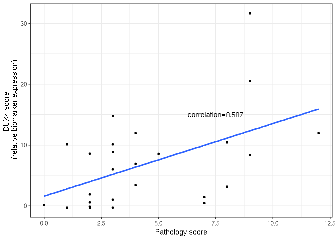

Figure 3.3: Scatter and linear regression of DUX4 and pathology score.

3.5.2 DUX4 and STIR signal

DUX4 score and qualitative T2-STIR rating of the follow-up biopsied FSHD muscles show moderate correlation (0.53).

cor <- cor(as.numeric(time_2$STIR_rating), time_2$DUX4.Score,
           method="spearman")
ggplot(time_2, aes(x=as.numeric(STIR_rating), y=DUX4.Score))+
  geom_point(size=1) +
  geom_smooth(method = lm, se=FALSE) + 
  annotate("text", x=2.5, y=14.5, vjust=0.5, 
           label=paste0("correlation=", format(cor, digits=3))) +
  theme_bw() +
  labs(y="DUX4 score \n (relative biomarker expression)",
       x="STIR rating")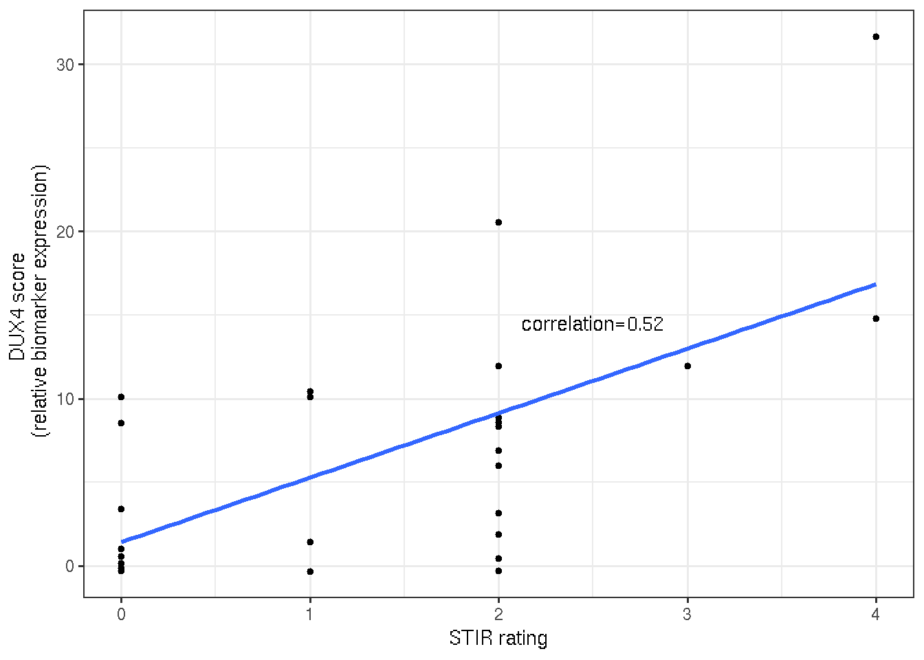

Figure 3.4: Scatter and linear regression plot of DUX4 socre and STIR rating.

72% of STIR-positive muscle biopsies show elevated DUX4 target expression (DUX4 score > 2.5).

DUX4_threshold <- 2.5 # an arbitrary threshold
#' adding new columns indicating DUX4 (+/-) 
#' if STIR = 0 but T1_rating > 0, than STIR_status should be NA, not MRI normal
new_time_2 <- time_2 %>%
  mutate(STIR_status = ifelse(STIR_rating > 0, "STIR+", "MRI normal")) %>%
  mutate(DUX4_status = ifelse(DUX4.Score > DUX4_threshold, "DUX4+", "DUX4-")) %>%
  mutate(STIR_status = ifelse((STIR_rating == 0 & T1_rating > 0), NA, STIR_status)) %>%
  dplyr::filter(!is.na(STIR_status))

gg_stir <- ggplot(new_time_2, aes(x=STIR_status, y=DUX4.Score,
                       group=STIR_status)) +
  geom_boxplot(outlier.shape = NA, width=0.5 ) +
  geom_jitter(width=0.2, size=1) +
  geom_hline(yintercept = DUX4_threshold, color="grey", 
             linetype="dashed") +
  theme_bw() + 
  labs(title="MRI normal vs. STIR+",
       y="DUX4 score", x="STIR status")  +
  theme(plot.title = element_text(size=9, hjust = 0.5))
gg_stir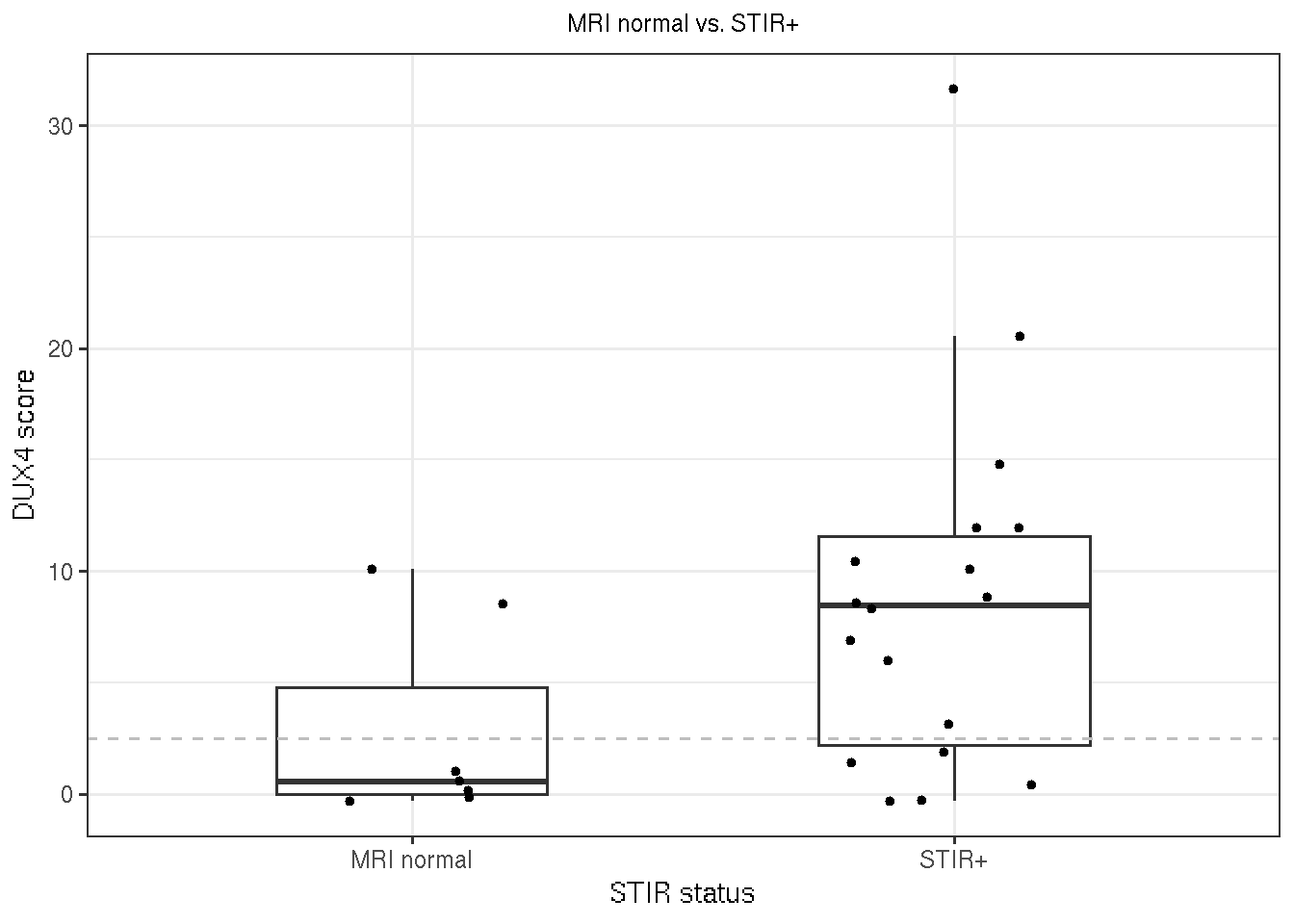

Figure 3.5: Boxplot of DUX4 scores by MRI status (normal and STIR+). The grey deshed line is where DUX4 score=2.5.

#new_time_2 %>% dplyr::filter(STIR_status == "MRI Normal")
message("DUX4 score mean/sd by STIR status")

## DUX4 score mean/sd by STIR status

new_time_2 %>% group_by(STIR_status) %>% summarize(avg=mean(DUX4.Score), sd=sd(DUX4.Score))

## # A tibble: 2 x 3
##   STIR_status   avg    sd
##   <chr>       <dbl> <dbl>
## 1 MRI normal   2.85  4.46
## 2 STIR+        8.69  8.05

message("Frequency of STIR+ with DUX4+ (DUX4 score > 2.5)")

## Frequency of STIR+ with DUX4+ (DUX4 score > 2.5)

new_time_2 %>% dplyr::filter(STIR_status == "STIR+") %>%
  summarize(freq = sum(DUX4_status == "DUX4+") / dplyr::n()) #18

##        freq
## 1 0.7222222

3.6 DUX4 score and T1 fat fraction

DUX4 score and T1 fat fraction seem poorly correlated in terms of linear regression, however, the mid-range of T1 fat fraction (0.2 ~ 0.4) displays a more positive relationship with the DUX4 score.

cor <- cor(time_2$fat_fraction, time_2$DUX4.Score, method="spearman")
ggplot(time_2, aes(x=fat_fraction, y=DUX4.Score))+
  geom_point(size=1) +
  geom_smooth(method = lm, se=FALSE) + 
  annotate("text", x=0.5, y=10, vjust=0.5, 
           label=paste0("correlation=", format(cor, digits=3))) +
  theme_bw() +
  labs(y="DUX4 score \n (relative biomarker expression)",
       x="T1 fat fraction")

$Scatter and linear regressio plot of DUX4 score and T1 fat fraction.$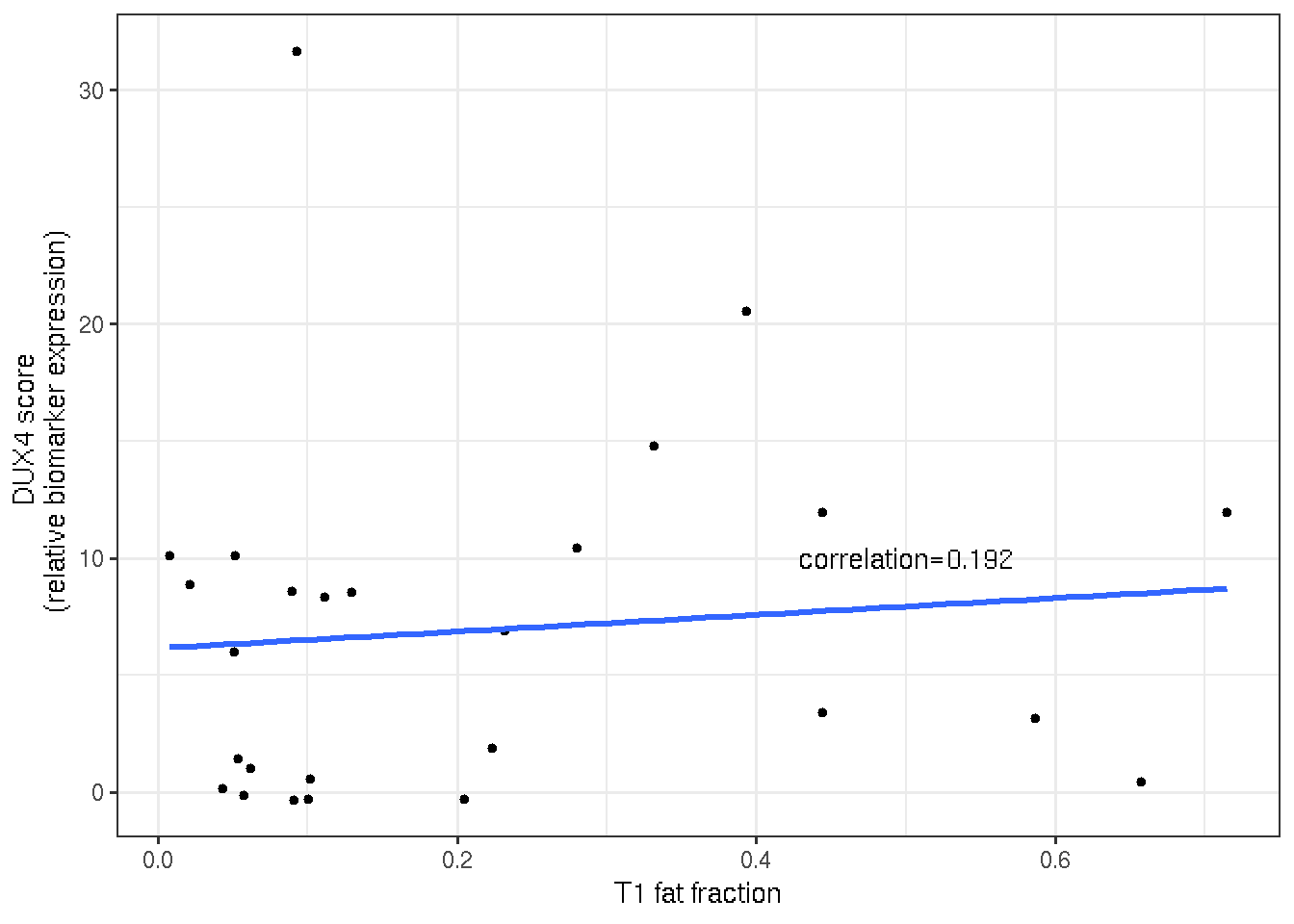

Figure 3.6: Scatter and linear regressio plot of DUX4 score and T1 fat fraction.

ggplot(time_2, aes(x=fat_fraction, y=DUX4.Score))+
  geom_point(size=1) +
  geom_smooth(method = loess, se=FALSE) + 
  geom_vline(xintercept = 0.2, linetype="dashed", color="gray") +
  geom_vline(xintercept = 0.4, linetype="dashed", color="gray") +
  theme_bw() +
  labs(y="DUX4 score \n (relative biomarker expression)",
       x="T1 fat fraction")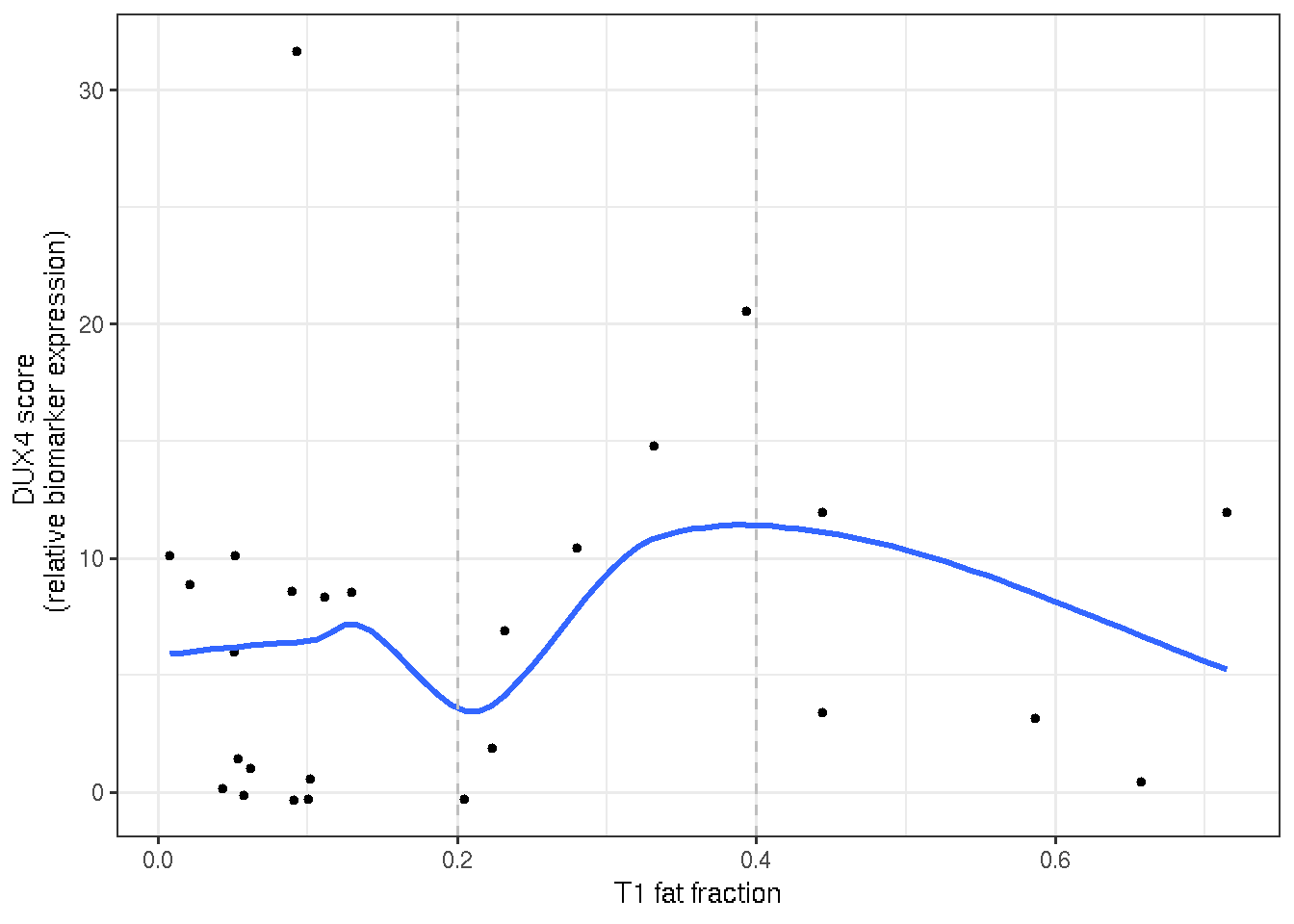

$Nonlinear relationship between DUX4 score and T1 fat fraction illustrates a positive relationship within the mid-range of T1 (0.2, 0.4)$

Figure 3.7: Nonlinear relationship between DUX4 score and T1 fat fraction illustrates a positive relationship within the mid-range of T1 (0.2, 0.4)

References

Love, Michael I., Wolfgang Huber, and Simon Anders. 2014. “Moderated Estimation of Fold Change and Dispersion for Rna-Seq Data with Deseq2.” Genome Biology 15 (12): 550. doi:10.1186/s13059-014-0550-8.

Yao, Zizhen, and et al. 2014. “DUX4-Induced Gene Expression Is the Major Molecular Signature in Fshd Skeletal Muscle.” Human Molecular Genetics. doi:10.1093/hmg/ddu251.