Chapter 6 Markers discriminate Mild FSHD from the control samples
The samples categorized as Mild FSHDs are characterized by low-to-absent DUX4-targeted gene expression, relatively low gene expression in all six relevant biological functions as well as lower pathological scores in average. We aim to find markers discriminating the Mild FSHD from the control samples, and these markers could be the early responsers to muscle changes and DUX4 regulation.
We first identify the differentially expressed (DE) genes in the Mild FSHDs relative to the controls, then keep the DE genes that are relevant to FSHD as candidate classifiers, or predictors. To assess the power of discrimination and perform cross-validation of the set, we apply Receiver Operator Characteristics (ROC) and random forests, respectively.
6.0.1 Load libaray and datasets
suppressPackageStartupMessages(library(DESeq2))
suppressPackageStartupMessages(library(tidyverse))
suppressPackageStartupMessages(library(pheatmap))
suppressPackageStartupMessages(library(ggplot2))
suppressPackageStartupMessages(library(BiocParallel))
multi_param <- MulticoreParam(worker=2)
register(multi_param, default=TRUE)

pkg_dir <- "/fh/fast/tapscott_s/CompBio/RNA-Seq/hg38.FSHD.biopsy.all"

source(file.path(pkg_dir, "scripts", "manuscript_tools.R"))
load(file.path(pkg_dir, "public_data", "cluster_df.rda"))
load(file.path(pkg_dir, "public_data", "sanitized.dds.rda"))
load(file.path(pkg_dir, "public_data", "sanitized.rlg.rda"))

sanitized.dds$RNA_cluster_5 <- sanitized.rlg$RNA_cluster_5 <- cluster_df$RNA_cluster
sanitized.dds$new_cluster_name <- sanitized.rlg$new_cluster_name <- cluster_df$new_cluster_name

#' DUX4-reguated 53 FSHD biomarkers
mk <- get(load(file.path(pkg_dir, "data", "FSHD_markers.rda")))$gene_name
mk <- mk[mk %in% rowData(sanitized.dds)$gene_name]
6.1 Differentially up-regulated genes in Mild FSHD samples
The criteria for differentially up-related gene in Mild FSHDs: adjusted \(p\)-value < 0.05 corresponding to \(H_0: |lfc| = 0\). Note that the difference in gene expression between the Mild FSHDs and controls is subtle, therefore a loosen criteria for the log fold change is applied.
#' tools
.tidy_results <- function(res, dds, padj_thres=0.05) {
  de <- as.data.frame(res) %>%
    rownames_to_column(var="gencode_id") %>%
    dplyr::filter(padj < padj_thres) %>%
    mutate(gene_name = rowData(dds[gencode_id])$gene_name) %>%
    mutate(gene_id =
             sapply(strsplit(gencode_id, ".", fixed=TRUE), "[[", 1))
}

#' DESeq2
#' class A vs A_control
new.dds <- sanitized.dds
design(new.dds) <- ~ RNA_cluster_5
new.dds <- DESeq(new.dds)
classA.res <- results(new.dds, alpha = 0.05,
                      name = "RNA_cluster_5_A_vs_A_Cntr")
de_A <- .tidy_results(classA.res, dds=new.dds, padj=0.05)
de_A_up <- de_A %>% dplyr::filter(log2FoldChange > 0) %>%
  mutate(DUX4_marker=gene_name %in% mk)
de_A_down <- as.data.frame(classA.res) %>%
  rownames_to_column(var="gene_id") %>%
  filter(padj < 0.05, log2FoldChange < 0) %>%
  mutate(gene_name=rowData(sanitized.dds[gene_id])$gene_name)
#'
#' class D vs A_control
#'
classD.res <- results(new.dds, alpha = 0.05, lfcThreshold=2,
                      name="RNA_cluster_5_D_vs_A_Cntr")
de_D_up <- .tidy_results(classD.res, dds=new.dds, padj=0.05) %>%
   dplyr::filter(log2FoldChange > 0) %>%
  mutate(DUX4_marker=gene_name %in% mk)
6.2 Select FSHD relavent candidates
We keep the up-regulated genes in the Mild FSHDs that are also robustly up-regulated in the High (cluster D) samples: adjusted \(p\)-value < 0.05 corresponding to \(H_0: |lfc| < 2\). This way we obtain the up-regulated genes in Mild FSHDs that are disease relevant. As a result, we obtain 164 candidates. Showing below is the row z-score of 164 candidates’ log expression in all samples.
#'
#' (1) select de_up that are robust in cluster D (High, lfc > 2 with padj < 0.05)
#' (2) define key predictors: limited to DE genes in High (class D)
#' (3) plot heatmap to see the progression of expression in other FSHD classes
#'
keys <- de_A_up %>% dplyr::filter(gencode_id %in% de_D_up$gencode_id) %>%
  arrange(padj)

keep <- sanitized.rlg$RNA_cluster_5 %in% c("A_Cntr", "A")

data <- assay(sanitized.rlg[keys$gencode_id, ])
rownames(data) <- keys$gene_name
ann_col <- data.frame(pheno_type=sanitized.rlg$pheno_type,
                      class = sanitized.rlg$RNA_cluster_5)
rownames(ann_col) <- colnames(data)
zscore_data <- (data - rowMeans(data)) / rowSds(data)
pheatmap(zscore_data, annotation_col=ann_col,
         #fontsize_row=6.5,
         #fontsize_col=6,
         scale="row",
         show_rownames=FALSE)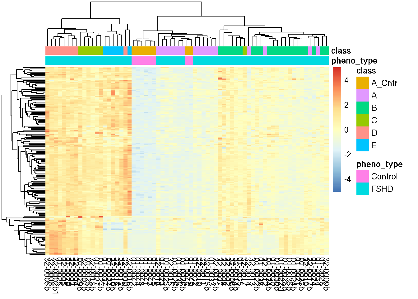
Figure 6.1: Heatmap of row z-score of 164 candidate log expression.
6.3 GO analysis
The top 10 enriched GO terms corresponding to the 164 early responser candidates are:
universal <- sapply(strsplit(rownames(classA.res), ".", fixed=TRUE),
                    "[[", 1)
enriched <- .do_goseq(universal = universal,
                      selected_genes = keys$gene_id,
                      return.DEInCat=FALSE, dds=sanitized.dds)
## Warning in pcls(G): initial point very close to some inequality constraintsknitr::kable(enriched[1:10, c("category", "term", "padj")],
caption = "Top 10 enriched GO terms correspoding to 163 candidates.")| category | term | padj |
|---|---|---|
| GO:0006952 | defense response | 0e+00 |
| GO:0009605 | response to external stimulus | 0e+00 |
| GO:0006954 | inflammatory response | 0e+00 |
| GO:0002684 | positive regulation of immune system process | 0e+00 |
| GO:0050776 | regulation of immune response | 0e+00 |
| GO:0050778 | positive regulation of immune response | 0e+00 |
| GO:0006955 | immune response | 0e+00 |
| GO:0002253 | activation of immune response | 0e+00 |
| GO:0002682 | regulation of immune system process | 1e-07 |
| GO:0008283 | cell proliferation | 1e-07 |
6.4 Cross validation by random forests
We use a random forest to determine the top 25 potentially the strongest candidates.
# make expset and load ML library
suppressPackageStartupMessages(library(randomForest))
suppressPackageStartupMessages(library(MLInterfaces))
## Warning: replacing previous import 'BiocGenerics::var' by 'stats::var' when
## loading 'MLInterfaces'suppressPackageStartupMessages(library(ROC))
suppressPackageStartupMessages(library(genefilter))
set.seed(123)
keep <- sanitized.rlg$RNA_cluster_5 %in% c("A_Cntr", "A")
tmp.dds <- sanitized.dds[keys$gencode_id, keep]
data <- .get_local_rlg(keys$gencode_id, tmp.dds)
rownames(data) <- rowData(tmp.dds[rownames(data)])$gene_name
#rownames(data) <- keys$gene_name
exp_set <- ExpressionSet(data,
phenoData = AnnotatedDataFrame(as.data.frame(colData(tmp.dds))))
# testing on one random forest in which the 32-xxxx samples are the testing set)
# obtaining potential best candidates accessed by random forests
train_ind <- c(1:11, 14:19)
rf1 <- MLearn(pheno_type ~., data=exp_set,
randomForestI, train_ind, ntree=1000, mtry=10, importance=TRUE)
imp <- getVarImp(rf1) # rownames are messed up by MLearn
rownames(imp) <- featureNames(exp_set)
tmp_data <- report(imp, n=25) %>%
arrange(MnDecrAcc) %>%
mutate(names=as.character(names)) %>%
mutate(names=factor(names, levels=names))
gg_imp <- ggplot(tmp_data, aes(x=names, y=MnDecrAcc)) +
geom_bar(stat="identity") +
coord_flip() +
theme_bw()
imp_data <- as.data.frame(imp@.Data) %>%
rownames_to_column(var="gene_name") %>%
#left_join(keys, by="gene_name") %>%
arrange(desc(MeanDecreaseAccuracy)) gg_imp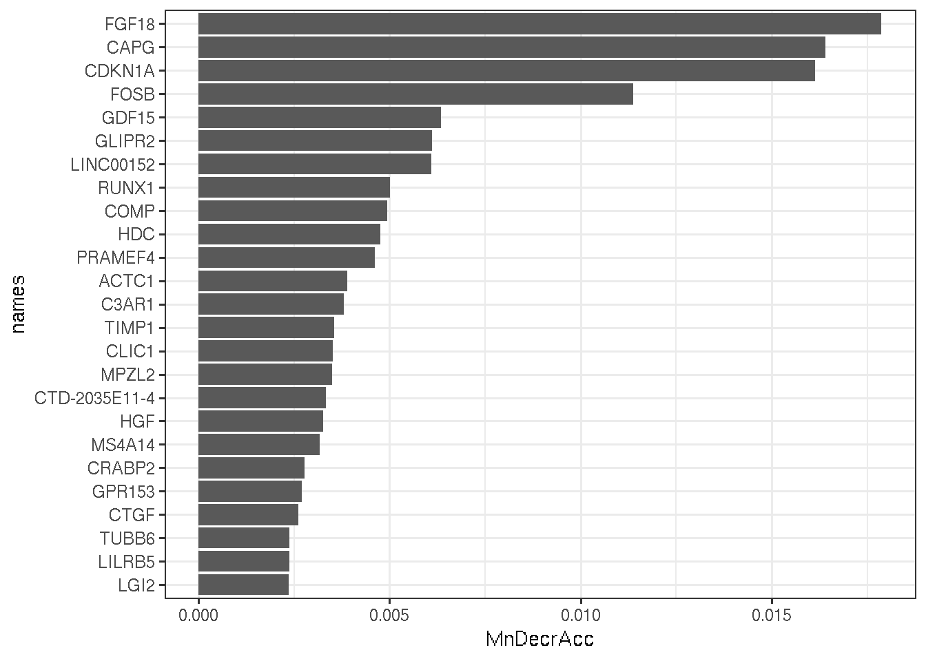
Figure 6.2: top 25 best candidates determined by a random forest.
Leave-one-out cross-validation by random forest yields 0.08 prediction error rate.
#' leave-one-out cross-validation
error_test <- lapply(1:ncol(exp_set), function(i) {
  train_ind <- c(1:25)[-i]
  rf <- MLearn(pheno_type ~., data=exp_set,
              randomForestI, train_ind, ntree=1000, mtry=10, importance=TRUE)
  cfm <- confuMat(rf, "test")
  error_sample <- ifelse(is.table(cfm), 1, 0)
})
error_rate <- sum(unlist(error_test)) / ncol(exp_set)
error_rate
## Samples
## 0.086.5 Discriminative power per candidates
Estimate discriminative power for individual genes using ROC.
rocs <- rowpAUCs(exp_set, "pheno_type", p=0.2)
rocs_data <- data.frame(pAUC = area(rocs), AUC = rocs@AUC) %>%
  rownames_to_column(var="gene_name")
# combine ROC and random forests results
comb_data <- left_join(imp_data, rocs_data, by="gene_name") %>%
  #dplyr::filter(pAUC > 0.1) %>%
  dplyr::select(-Control, -FSHD, -MeanDecreaseGini) %>%
  left_join(keys %>% dplyr::select(-c(gencode_id, gene_id)), by="gene_name")
6.6 Heatmap of some best candidates
Here we select 52 candidates (out of 164) with \(AUC > 0.9\)) as our discovery set as early responser to muscle changes are best in discriminating mildly affect FSHDs from the controls.
predictors <- comb_data %>% dplyr::filter(AUC >= 0.9) %>%
  mutate(gencode_id = get_ensembl(gene_name, sanitized.dds)) %>%
 pull(gencode_id) #52

keep <- sanitized.rlg$RNA_cluster_5 %in% c("A_Cntr", "A")
tmp.dds <- sanitized.dds[predictors, keep]
#data <- assay(tmp.rlg)
data <- .get_local_rlg(predictors, tmp.dds)
rownames(data) <- rowData(tmp.dds)$gene_name
ann_col <- data.frame(pheno_type=tmp.dds$pheno_type,
                      class = tmp.dds$RNA_cluster_5)
rownames(ann_col) <- colnames(data)
zscore_data <- (data - rowMeans(data)) / rowSds(data)
pheatmap(zscore_data, annotation_col=ann_col,
         fontsize_row=6.5,
         #fontsize_col=6,
         scale="row",
         show_rownames=TRUE,
         cellheight=8)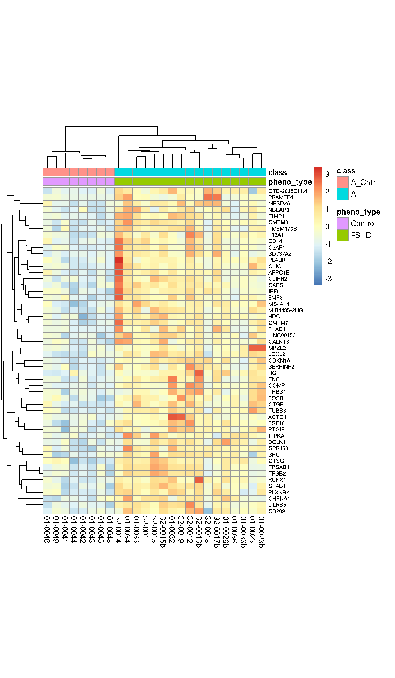
Figure 6.3: 52 early muscle change candidates with AUC > 0.9.
6.7 Some strong candidates
6.7.1 CKDN1A
CDKN1A is one of the best candidates in terms of AUC and pAUC (p=0.2). Shown below are its \(\log_{10}(TPM)\) expression and ROC statistics and AUC plot.
sel <- c("CDKN1A", "C1QA", "CD4", "TNC", "RUNX1", "LILRB5", "FGF18", "CCL18")
factor <- as.character(cluster_df$new_cluster_name)
factor[cluster_df$RNA_cluster=="A_Cntr"] <- "Control"
factor <- factor(factor, levels=c("Control", "Mild", "Moderate", "IG-High", "High", "Muscle-Low"))
names(factor) <- as.character(cluster_df$sample_name)

set_exp <- .getExpFromDDS_by_cluster(sel, dds=sanitized.dds, factor=factor, type="TPM")
## Warning: `as.tibble()` is deprecated, use `as_tibble()` (but mind the new semantics).
## This warning is displayed once per session.data <- set_exp %>%
mutate(log.value=log10(value+1))
gg_CDKN1A <- ggplot(data %>% filter(gene_name=="CDKN1A"),
aes(x=group, y=log.value, group=group)) +
geom_boxplot(outlier.shape = NA, width=0.7) +
#geom_violin() +
geom_jitter(width=0.2, size=0.8) +
labs(y=bquote(log[10]~"(TPM+1)"), title="CDKN1A") +
theme_bw() +
theme(axis.text.x=element_text(angle=90, vjust=0.5, hjust=1),
axis.title.x = element_blank(),
plot.title = element_text(hjust=0.5, size=10),
axis.title.y = element_text(size=9),
legend.justification=c(0,1), legend.position=c(0, 1))
gg_CDKN1A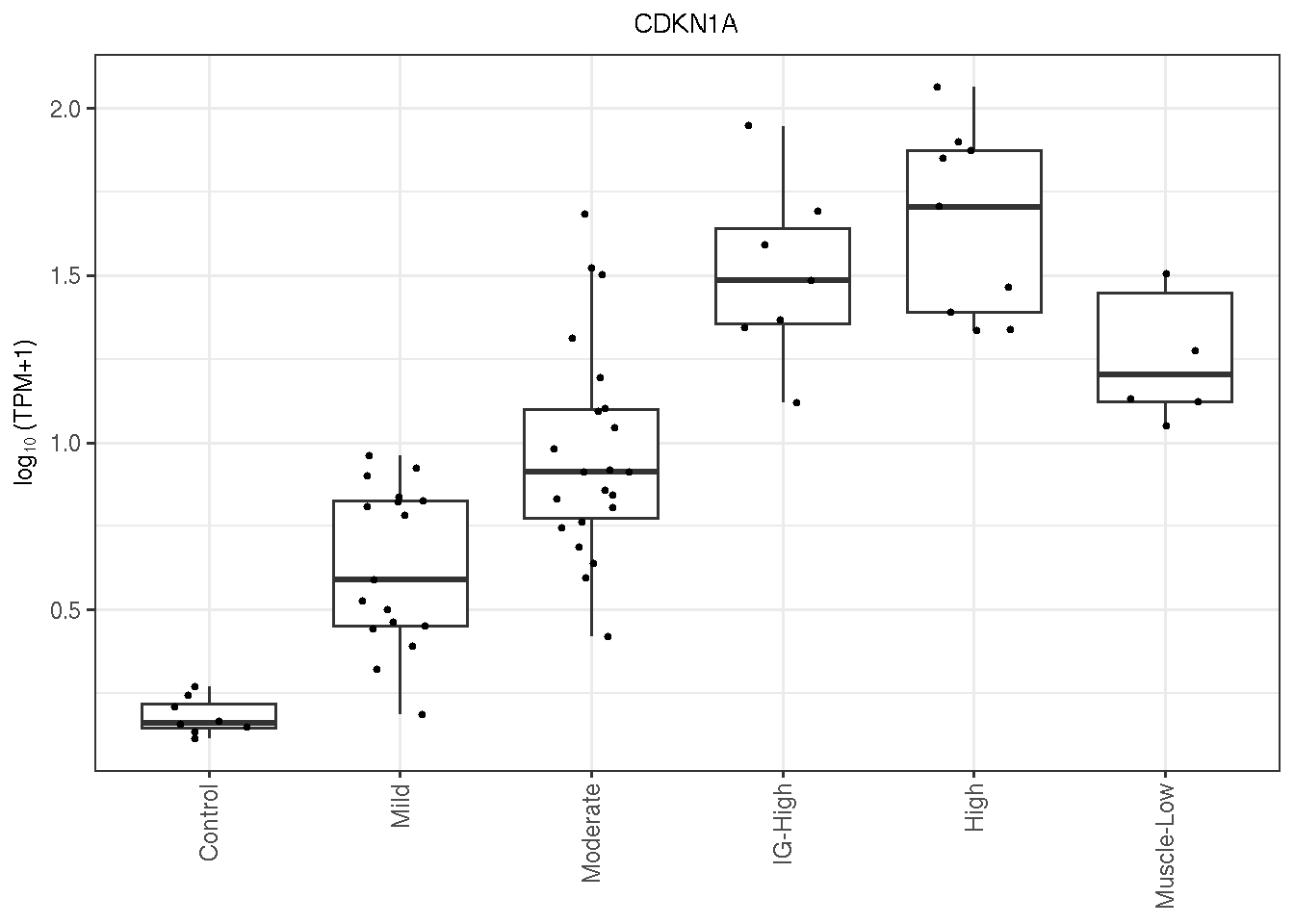
plot(rocs["CDKN1A"], main="CDKN1A")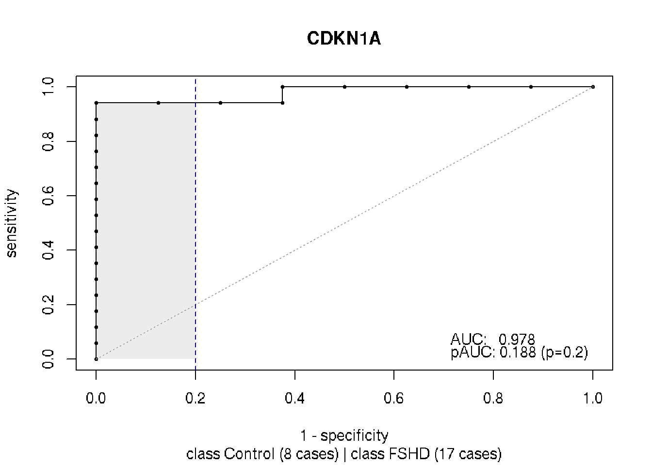
6.7.2 CCNA1
CCNA1 is a DUX4-regulated genes and a great candidate for discriminating Mild FSHDs from the controls. Below is its \(\log_{10}(TPM)\) expression by FSHD classes.
ccna1_exp <- .getExpFromDDS_by_cluster("CCNA1", dds=sanitized.dds, factor=factor, type="TPM")
data <- ccna1_exp %>%
  mutate(log.value=log10(value+1))
gg_CCNA1 <- ggplot(data %>% filter(gene_name=="CCNA1"),
                   aes(x=group, y=log.value, group=group)) +
    geom_boxplot(outlier.shape = NA, width=0.7) +
    #geom_violin() +
    geom_jitter(width=0.2, size=0.8) +
    labs(y=bquote(log[10]~"(TPM+1)"), title="CCNA1") +
    theme_bw() +
    theme(axis.text.x=element_text(angle=90, vjust=0.5, hjust=1),
          axis.title.x = element_blank(),
          plot.title = element_text(hjust=0.5, size=10),
          axis.title.y = element_text(size=9),
          legend.justification=c(0,1), legend.position=c(0, 1))
gg_CCNA1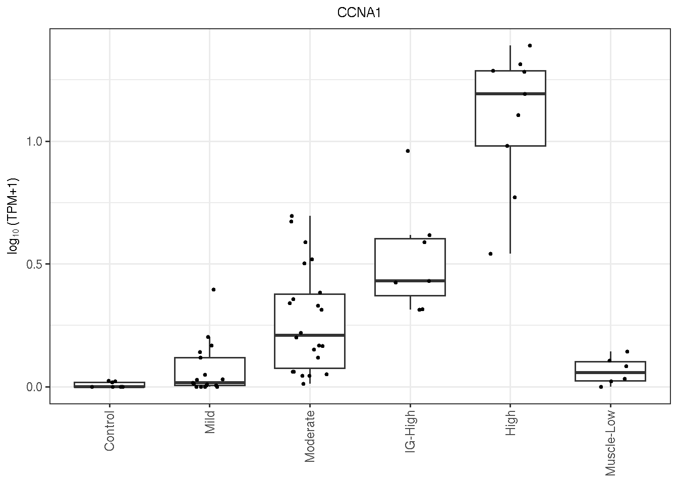
CCNA1’s ROC plot and results.
plot(rocs["CCNA1"], main="CCNA1")
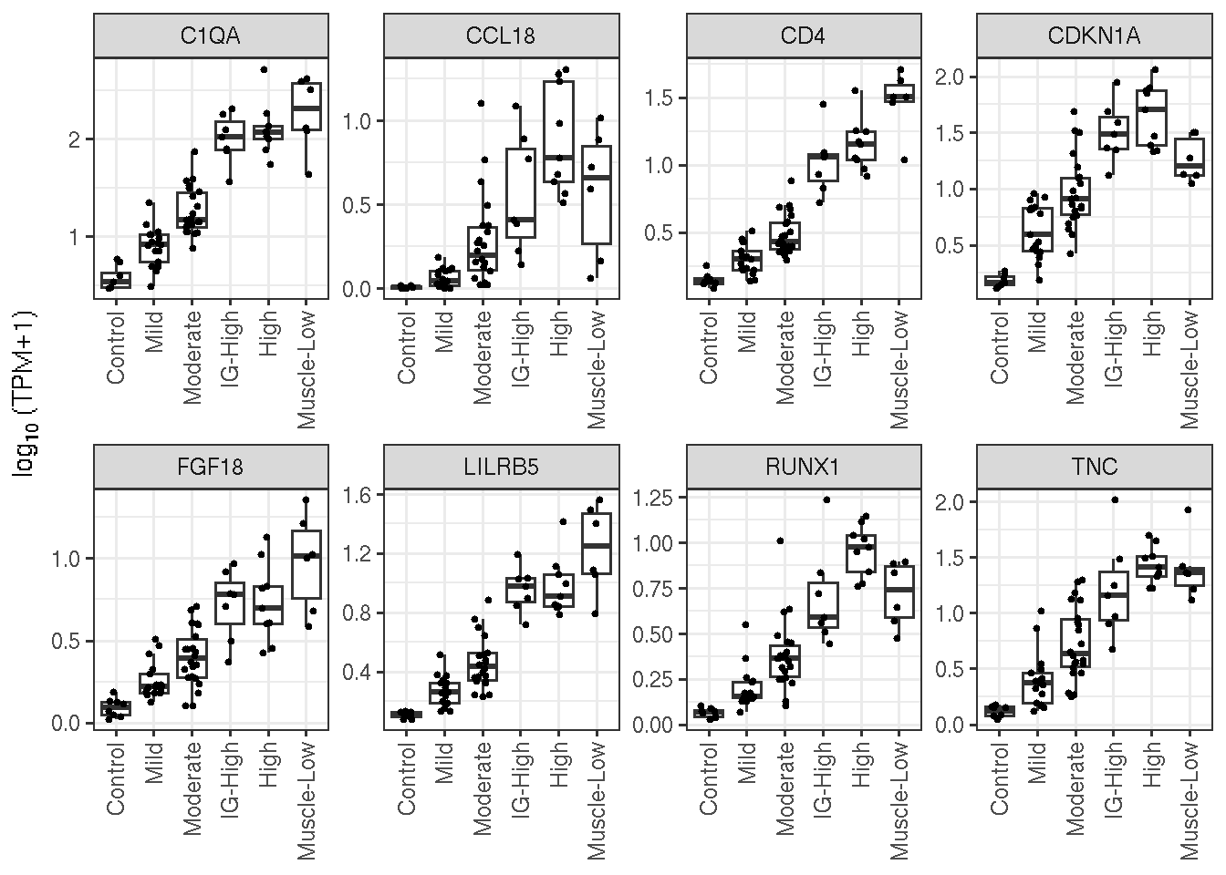
6.7.3 And few more examples
Some strong candidates’ \(\log_{10}TPM\) expression by FSHD classes.
data <- set_exp %>%
  mutate(log.value=log10(value+1))
ggplot(data, aes(x=group, y=log.value, group=group)) +
    geom_boxplot(outlier.shape = NA) +
    geom_jitter(width=0.2, size=0.7) +
    facet_wrap( ~ gene_name, nrow=2, scale="free") +
    theme_bw() +
    labs(y=bquote(log[10]~"(TPM+1)")) +
    theme(axis.text.x=element_text(angle=90, vjust=0.5, hjust=1),
          axis.title.x = element_blank(),
          legend.justification=c(0,1), legend.position=c(0, 1))