Chapter 6 Repeat elements
In this chapter, we performed repeat element profiling and inferred repeat family and class activation in CinC and HinC transcriptome using gene set enrichment analysis (GSEA). The computational methods we employed include
- counting reads that overlap with repeat elements
- identifing DUX4/DUXC affected repeat elements by DESeq2
- comparing CinC to HinC repeats profiling
- analying family and class enrichment in repeat elements
- estimating peaks distribution in class of repeat elements
the following chapters, 7 and 8, investigated more detials of retrotransposons and satellite repeats. (regulatory activities in our canine model and the impact in DUXC and DUX4 expressed canine muscles.)
6.1 Takeaway
The RNA expression levels of repeat elements in DUXC expressed muscle cells is highly correlated with that in DUX4 (Pearson=0.782). We used the repeats annotation from UCSC Repeat Masker (RMSK) track on main chromosomes of canFam3 genome. With a threshold of adjusted \(p\)-value < 0.05 corresponding to the null hypothesis \(H_0: |log2FC| < 1\), DESeq2 identified 231 and 99 differentially expressed repeat elements in DUX4 and DUXC expressed canine skeletal cells, respectively, compared with the cells expressing Luciferase. 86% (83/99) of the differentially expressed repeat elements in CinC is overlapped with that of in HinC.
DUX4 continued to show the trend of activating retrotransposons as it did in human skeletal muscle (Jennifer L. Whiddon 2017) and in the 2C-like embryonic stage (Peter G Hendrickson 2017). Similarly, DUXC followed the same trend in canine. In fact, by gene set enrichment analysis using hypergeometric tests (code shown below), LINE1, ERV1, ERVL, and ERVL-MaLR LTR subfamilies were enriched in both DUX4 and DUXC expressed canine skeletal muscle. Almost all the activated LTRs of DUXC were overlapping with that of DUX4. Moreover, the peak binding distribution in classes of repeat element confirmed the preference of DUX4 and DUXC in binding to LTRs and LINE1: LTRs and LINEs constitute 5% and 15% of the reference canine genome, respectively, whereas the frequency of the peak binding sites (within +/- 50 from the summit) on LTRs and LINEs are 14% ~ 17% and 21% ~ 35%, respectively. The enrichment of LTRs activation is statistically significant. But the evidence of DUXC’s direct activation to LINE1 remains subtle and requires further investigation (e.g. motifs of peaks that bind to LINE1).
Load libraries and datasets
suppressPackageStartupMessages(library(TxDb.Cfamiliaris.UCSC.canFam3.ensGene))
suppressPackageStartupMessages(library(canFam3.rmsk))
suppressPackageStartupMessages(library(tidyverse))
suppressPackageStartupMessages(library(wesanderson) )
suppressPackageStartupMessages(library(DESeq2))
suppressPackageStartupMessages(library(latex2exp))

pkg_dir <- "~/CompBio/canFam3.DuxFamily"
fig_dir <- file.path(pkg_dir, "figures")
data_dir <- file.path(pkg_dir, "data")

load(file.path(pkg_dir, "data", "peaks_list.rda"))
load(file.path(pkg_dir, "data", "rmsk.dds.rda"))
load(file.path(pkg_dir, "data", "CinC.ens.dds.rda"))
load(file.path(pkg_dir, "data", "HinC.ens.dds.rda"))
load(file.path(pkg_dir, "data", "CALTinC.ens.dds.rda"))

source(file.path(pkg_dir, "scripts", "tools.R"))
6.2 Repeat element expression
The repeat elements we used here were collected from UCSC’s Repeat Masker (RMSK) annotation track. We estimated the repeat elements expression by counting the reads that overlap the instances of repeat elements (featured by RMSK’s repName); each read count was adjusted by its number of reported multiple alignments (column NH, BAM format). The fractional counts were then rounded and saved as an DESeqDataSet instance (/data/rmsk.dds.rda)
The countHits() function, code shown beloww, performed the counting; it is only being tested for single-ended RNA-seq reads (see /scripts/summarizeOverlaps.adjNH.R).
# summarizeOverlaps-adjNH(features, all.reads)
.countSubjectHits.2 <- function(ov, features, reads) {
    fracReadCount <- reads[queryHits(ov)]$count/reads[queryHits(ov)]$NH
    cnt <- rep(0, length(features))
    names(cnt) <- names(features)
    tmp <- tapply(fracReadCount, subjectHits(ov), sum)
    cnt[as.integer(names(tmp))] <- tmp
    as.integer(round(cnt))
}

countHits <- function(features, reads, type=c("any", "start", "end", "within"),
                  ignore.strand=TRUE, inter.feature=FALSE)
{   ## feathers is GRangeList containing repName's range data (importd from the canFam.rmsk package)
    ## reads is GAlignment instance - see GenomicAlignments package
    ov <- findOverlaps(reads, features, type=match.arg(type),
                       ignore.strand=ignore.strand)
    if (inter.feature) {
        ## Remove ambigous reads.
        reads_to_keep <- which(countQueryHits(ov) == 1L)
        ov <- ov[queryHits(ov) %in% reads_to_keep]
    }
    .countSubjectHits.2(ov, features=features, reads=reads)
}
6.3 Differential analysis
Aims
- Compare DUXC (CinC) and DUX4 (HinC) expressed cell lines with Luciferase expressed
- Identify targets of DUXC and DUX4 in repeat elements
6.3.1 Normalization
Prior to differential analysis, we needed to set appropriate, unbiased size factor for each sample. DUXC and DUX4 tend to activate retrotransponsons and result much more repeat element transcripts than that of Luciferase. So merely using the number of repeat elements trasncripts for size factors would magnify the normalized expression induced by Luciferase. Therefore we used the size factors estimated by DESeq2 over the total transcripts (all gene features).
6.3.2 DESeq2 results
Differentially expressed repeat elements (featured by repName) were called if adjusted \(p\)-value \(< 0.05\), corresponding to null hypothesis \(H_0:|log2FC| < 1\). Among ~ 700 annotated repeat elements, the DESeq2 analysis resulted 231 and 99 differentially up-regulated repeat elements in HinC and CinC models, respectively. Code and MA plots are shown below.
Adjust size factors
new_rmsk_dds <- lapply(names(rmsk.dds), function(name) {
  # use size factor estimated over total transcripts
  dds <- rmsk.dds[[name]]

    if (name == "CinC")
      sizeFactors(dds) <- sizeFactors(CinC.ens.dds)

    if (name == "HinC")
      sizeFactors(dds) <- sizeFactors(HinC.ens.dds)

    if (name == "CALTinC")
      sizeFactors(dds) <- sizeFactors(CALTinC.ens.dds)

    dds <- DESeq(dds)

    return(dds)
})
names(new_rmsk_dds) <- names(rmsk.dds)
Make MA plots
# MA plots for CinC and HinC
lapply(names(new_rmsk_dds[1:2]), function(name) {
    # make MA plots
    dds <- new_rmsk_dds[[name]]
    res <- results(dds, alpha=0.05, lfcThreshold = 1)
    summary <- as(res, "data.frame") %>%
      summarise(up = sum(padj < 0.05 & log2FoldChange > 1, na.rm=TRUE),
      down = sum(padj < 0.05 & log2FoldChange < 1, na.rm=TRUE))

    file_name <- paste0("rmsk_", name, "_MAplot.pdf")
    y_text <- c(down=-4, up=4)

    if (name == "CinC") y_text <- c(down=-2, up=2)

    #pdf(file.path(fig_dir, file_name), height=4, width=4.5)
    plotMA(res, alpha = 0.05,
           main=paste0(name, ": ", nrow(res), " annotated elements"))
    label <- sprintf("LFC > 1 (up) : %d, %1.1f%%",
                     pull(summary, up), pull(summary, up)/nrow(res) *100)
    text(x=80, y=y_text["up"],   labels=label, adj=c(0, 0))
    label <- sprintf("LFC < 1 (down) : %d, %1.1f%%",
                     pull(summary, down), pull(summary, down)/nrow(res) *100)
    text(x=80, y=y_text["down"], labels=label, adj=c(0, 1))
    #dev.off()
})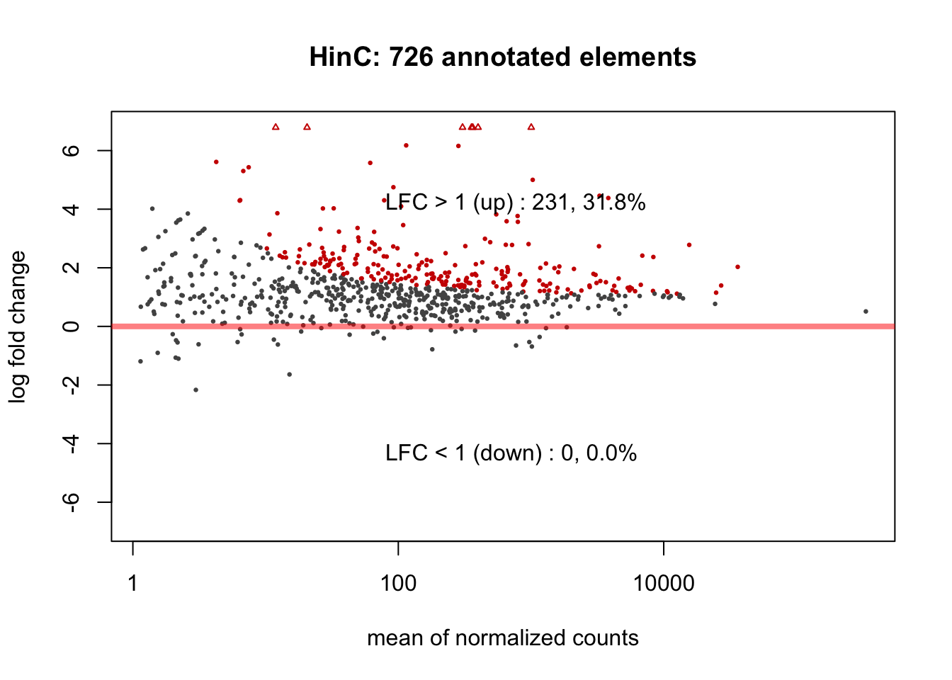
Figure 6.1: MAPlots of DESeq2 results for HinC and CinC transcriptome.
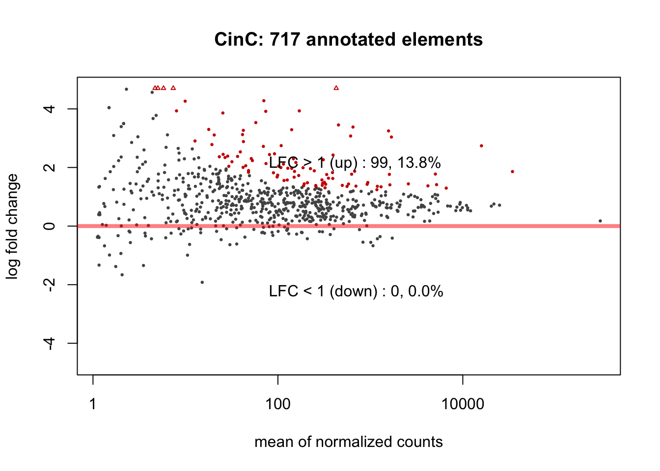
Figure 6.2: MAPlots of DESeq2 results for HinC and CinC transcriptome.
## [[1]]
## NULL
##
## [[2]]
## NULL
6.4 Repeat family enrichment analysis
To inferr which repeat family or class is enriched (compared with luciferase), we implemented gene set enrichment analysis (GSEA) using hypergeometric tests (see /scripts/tools.R). The .rmsk_enrichment() function below returned both the DESeq2 and GSEA results.
.rmsk_enrichment <- function(rmsk_dds) {
    # DESeq2 threshold: p-value=0.05 correspondng to H_0: |lfc| < 1
    rowdata <- as(rowData(rmsk_dds), "data.frame") %>%
      rownames_to_column(var="repName") %>%
      dplyr::select(repName, repClass, repFamily)
    # results using designated threshold and null hypothesis
    res_df <- as(results(rmsk_dds, alpha=0.05, lfcThreshold=1), "data.frame") %>%
      rownames_to_column(var="repName") %>%
      left_join(rowdata, by="repName")

    universe <- nrow(res_df)
    selected_up <- res_df %>%
      summarise(up = sum(padj < 0.05 & log2FoldChange > 0, na.rm=TRUE)) %>%
      pull(up)
    selected_down <- res_df %>%
      summarise(down = sum(padj < 0.05 & log2FoldChange < 0, na.rm=TRUE)) %>%
      pull(down)

    # repFamily enrichment/depletion summary
    repFamily_summary <- res_df %>% group_by(repFamily) %>%
      summarise(total=dplyr::n(),
                up = sum(padj < 0.05 & log2FoldChange > 0, na.rm=TRUE),
                down = sum(padj < 0.05 & log2FoldChange < 0, na.rm=TRUE),
                enrichment_prob = dhyper(x=up, k=total, m=selected_up, n=universe - selected_up),
                enrichment_mu = total * selected_up/universe)
                #depletion_prob = dhyper(x=down, k=total, m=selected_down,
                #                        n=universe-selected_down),
                #depletion_mu = total * selected_down/universe)

    # repClass enrichement/depletion summary
    repClass_summary <- res_df %>% group_by(repClass) %>%
       summarise(total=dplyr::n(),
                up = sum(padj < 0.05 & log2FoldChange > 0, na.rm=TRUE),
                down = sum(padj < 0.05 & log2FoldChange < 0, na.rm=TRUE),
                enrichment_prob = dhyper(x=up, k=total, m=selected_up, n=universe - selected_up),
                enrichment_mu = total * selected_up/universe)
    return(list(res_df=res_df,
                repFamily_summary=repFamily_summary,
                repClass_summary=repClass_summary))
}
Calling .rmsk_enrichement() and saving results HinC_rmsk.rda and CinC_rmsk.rda:
#source(file.path(pkg_dir, "scripts", "tools.R")) # .rmsk_enrichment
HinC_rmsk <- .rmsk_enrichment(new_rmsk_dds[["HinC"]])
## `summarise()` ungrouping output (override with `.groups` argument)
## `summarise()` ungrouping output (override with `.groups` argument)## `summarise()` ungrouping output (override with `.groups` argument)
## `summarise()` ungrouping output (override with `.groups` argument)## `summarise()` ungrouping output (override with `.groups` argument)
## `summarise()` ungrouping output (override with `.groups` argument)#save(HinC_rmsk, file=file.path(data_dir, "HinC_rmsk.rda"))
#save(CinC_rmsk, file=file.path(data_dir, "CinC_rmsk.rda"))
#save(CALTinC_rmsk, file=file.path(pkg_dir, "data", "CALTinC_rmsk.rda"))6.4.1 Correlation between HinC and CinC transcriptome
The CinC and HinC transcriptome are highly correlated - Pearson correlation is 0.782. 86% (83/99) of the differentially expressed repeat elements in CinC is overlapped with that of in HinC.
# (1c) scatter plot of HinC and CinC; highlight LTR: ERVL-MaLR
comb <- inner_join(HinC_rmsk$res_df, CinC_rmsk$res_df,
by="repName", suffix=c("_HinC", "_CinC")) %>%
dplyr::mutate(show_name = as.character(repFamily_HinC)) %>%
dplyr::mutate(show_name = ifelse(abs(log2FoldChange_HinC-log2FoldChange_CinC) < 1.5,
"", show_name)) %>%
dplyr::mutate(DE_status = "neither") %>%
dplyr::mutate(DE_status =
replace(DE_status, padj_HinC < 0.05 | padj_CinC < 0.05, "either")) %>%
dplyr::mutate(DE_status = replace(DE_status, padj_HinC < 0.05 & padj_CinC < 0.05, "both")) %>%
dplyr::mutate(DE_status = factor(DE_status, levels=c("neither", "either", "both")))
# label repeat family if |HinC - CInC lfc| > 1.5
library(ggrepel)
gg1 <- ggplot(comb, aes(x=log2FoldChange_CinC, y=log2FoldChange_HinC)) +
geom_point(size=1, alpha=0.7, aes(color=DE_status)) +
scale_color_manual(values=c("#999999","#E69F00", "#56B4E9")) +
geom_smooth(method="lm", se=FALSE, show.legend=FALSE, color="gray66",
alpha=0.5,
linetype="dashed") +
geom_abline(intercept=0, slope=1, color="gray25", alpha=0.2, size=0.5) +
labs(title=TeX("RMSK: HinC vs. CinC $\\log_2$ fold change"),
y=TeX("HinC: $\\log_2$(DUX4/luciferase)"),
x=TeX("CinC: $\\log_2$(DUXC/luciferase)"),
color="Differentially expressed") +
theme_bw()+
theme(legend.position = c(0.8, 0.14),
plot.title = element_text(hjust = 0.5, face="bold", size=14),
legend.background = element_rect(colour = 'black', fill = 'white',
linetype='solid')) +
geom_text_repel(aes(label=show_name), size=3, show.legend=FALSE)
df <- comb %>% dplyr::select(log2FoldChange_HinC, log2FoldChange_CinC) %>%
rename(y=log2FoldChange_HinC, x=log2FoldChange_CinC)
gg1 <- gg1 + geom_text(x = 7.5, y = 7.5, vjust=0, hjust=0.5,
label = lm_eqn(df), parse = TRUE, color="gray25", alpha=0.5)
gg1 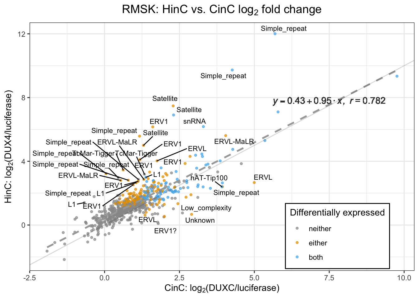
Figure 6.3: Scatter plot of repeat elements’ (repNAME) logFC in HinC and CinC with linear regression line (dashed line). The Pearson correlation is 0.782. Each dot represents a repeat element; an element’s repeat family is labelled if its difference between theå logFC in HinC and CinC is greater than 1.5.
suppressPackageStartupMessages(library(ggVennDiagram))
duxc_de <- CinC_rmsk$res_df %>% dplyr::filter(padj < 0.05)
dux4_de <- HinC_rmsk$res_df %>% dplyr::filter(padj < 0.05)
venn_data <- list(CinC = as.character(duxc_de$repName),
HinC = as.character(dux4_de$repName))
ggVennDiagram(venn_data) +
scale_fill_gradient(low="#E1AF00", high="#3B9AB2") +
labs(title="RMSK: differentially expressed elements")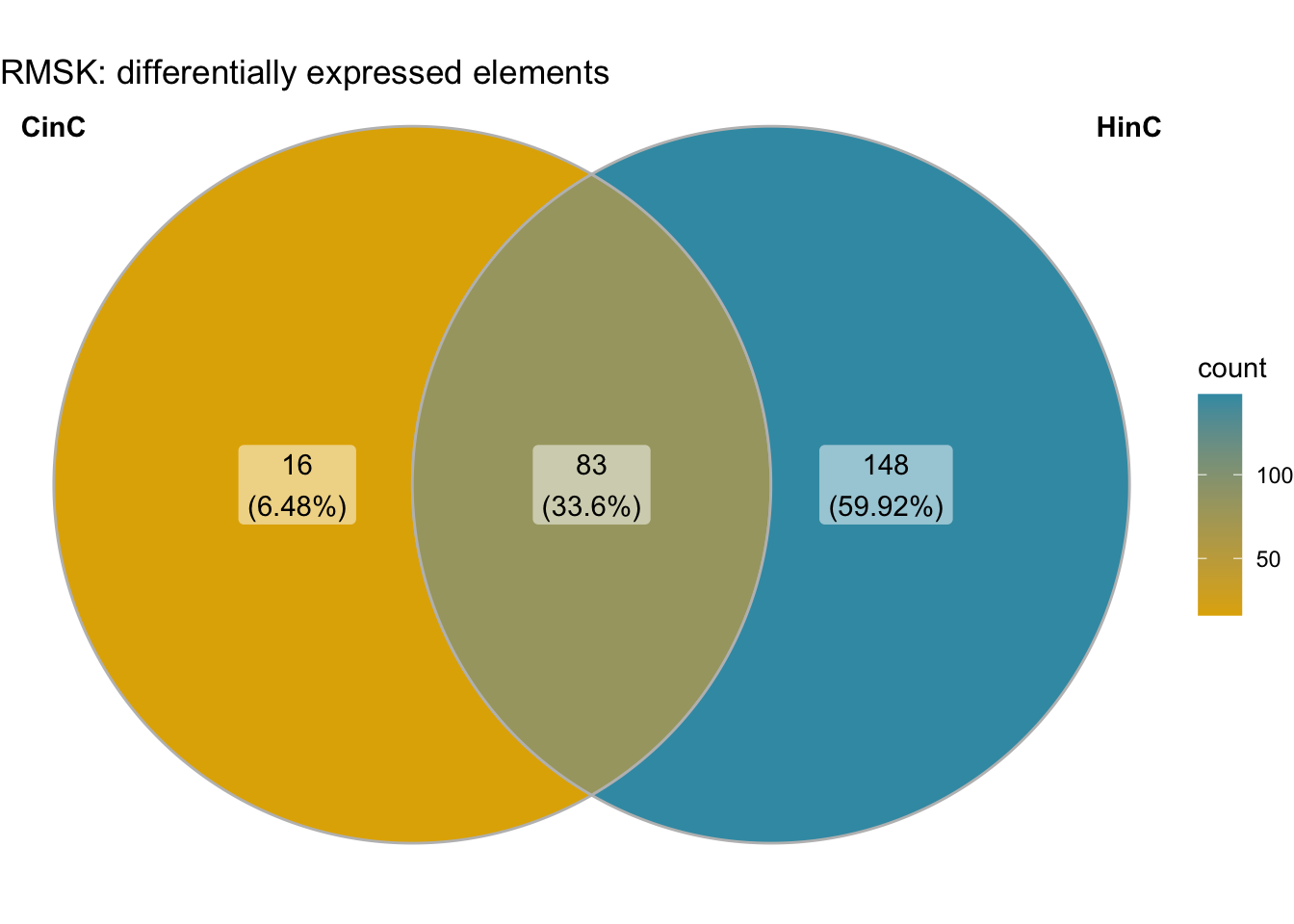
Figure 6.4: Venn diagram of differentially expressed repeat elements in CinC and HinC.
6.4.2 Repeat family activation
Among 48 families of repeat elements, ERVL subfamilies and LINE1 are over-represented in CinC and HinC trasncriptome: the number of up-regulated repeat elements in the family is higher than expected (by hypergeometric tests).
family_res <- full_join(HinC_rmsk$repFamily_summary, CinC_rmsk$repFamily_summary,
by="repFamily", suffix=c("_HinC", "_CinC")) %>%
dplyr::select(repFamily, enrichment_prob_HinC, enrichment_prob_CinC,
up_HinC, up_CinC, enrichment_mu_HinC, enrichment_mu_CinC) %>%
tidyr::gather(key="sample", value="pval", -repFamily,
-up_HinC, -up_CinC, -enrichment_mu_HinC, -enrichment_mu_CinC) %>%
dplyr::mutate(sample = ifelse(grepl("HinC", sample), "HinC", "CinC")) %>%
dplyr::mutate(log10Pval = -10*log10(pval)) %>%
dplyr::mutate(up = ifelse(sample=="HinC", up_HinC, up_CinC),
mu = ifelse(sample=="HinC", enrichment_mu_HinC, enrichment_mu_CinC)) %>%
dplyr::mutate(overrepresented = pval < 0.1 & up > mu)
gg <- ggplot(family_res, aes(x=repFamily, y=sample)) +
geom_point(aes(size=log10Pval, color=overrepresented, fill=overrepresented)) +
theme_minimal() +
theme(axis.text.x = element_text(angle = 90, hjust = 1, vjust=0.5),
axis.title.x=element_blank(),
axis.title.y=element_blank(),
legend.position="bottom",
plot.title = element_text(hjust = 0.5, face="bold", size=14)) +
labs(title=TeX("Repeat Family GSEA: $-10\\log_{10}(p-value)$"),
size=TeX("$-10\\log_{10}(p-value)$")) +
scale_fill_manual(name ="over-represented", values=c("ivory4", "firebrick4")) +
scale_color_manual(name="over-represented", values=c("ivory4", "firebrick4"))
gg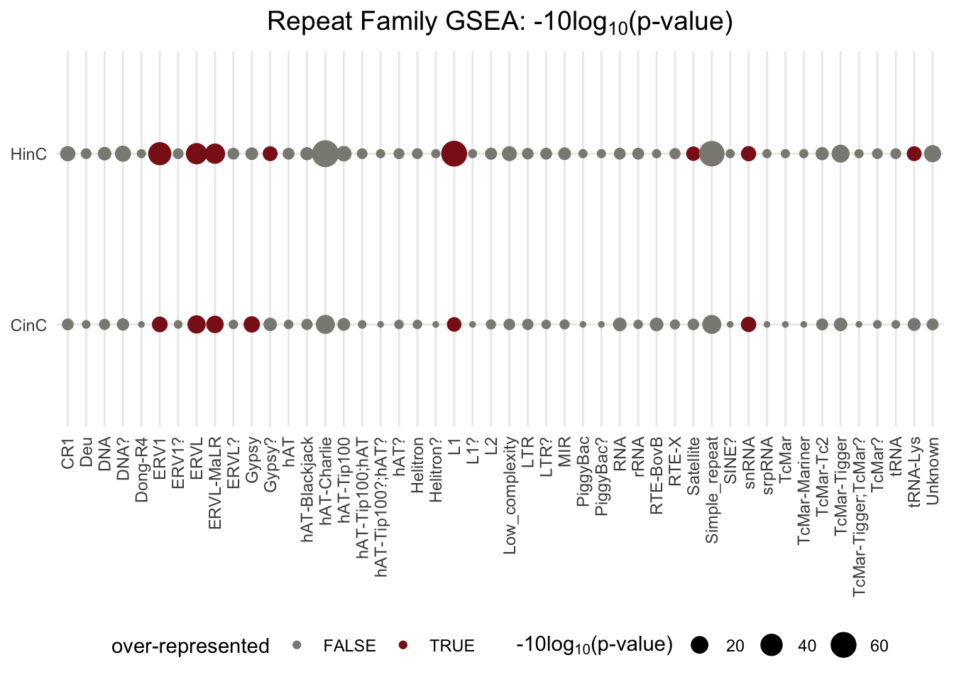
Figure 6.5: GSEA p-values in families of repeat elements. The p-value deteremines whether the number of up-regulated repeat elements in the family is different from expected; the size of dots reflect the scaled p-values, -10log10(p-value); red dots present over-represented families (p-value < 0.1 and the number of up-regulated elements is higher than expected).
6.4.3 Repeat classs activation
Similarily, using the same method above, LTR is determined activated (over-represetend).
class_res <- full_join(HinC_rmsk$repClass_summary, CinC_rmsk$repClass_summary,
by="repClass", suffix=c("_HinC", "_CinC")) %>%
dplyr::select(repClass, enrichment_prob_HinC, enrichment_prob_CinC,
up_HinC, up_CinC, enrichment_mu_HinC, enrichment_mu_CinC) %>%
tidyr::gather(key="sample", value="pval", -repClass,
-up_HinC, -up_CinC, -enrichment_mu_HinC, -enrichment_mu_CinC) %>%
dplyr::mutate(sample = ifelse(grepl("HinC", sample), "HinC", "CinC")) %>%
dplyr::mutate(log10Pval = -10*log10(pval)) %>%
dplyr::mutate(up = ifelse(sample=="HinC", up_HinC, up_CinC),
mu = ifelse(sample=="HinC", enrichment_mu_HinC, enrichment_mu_CinC)) %>%
dplyr::mutate(overrepresented = pval < 0.1 & up > mu)
gg <- ggplot(class_res, aes(x=repClass, y=sample)) +
geom_point(aes(size=log10Pval, color=overrepresented, fill=overrepresented), show.legend=FALSE) +
theme_minimal() +
theme(axis.text.x = element_text(angle = 90, hjust = 1, vjust=0.5),
axis.title.x=element_blank(),
axis.title.y=element_blank(),
legend.position="bottom") +
labs(title=expression("Repeat Class GSEA: " ~ -10 * Log[10] ~ "(p-value)"),
size = expression(-10 * Log[10] ~ "(p-value)")) +
scale_fill_manual(name ="over-represented", values=c("ivory4", "firebrick4")) +
scale_color_manual(name="over-represented", values=c("ivory4", "firebrick4"))
gg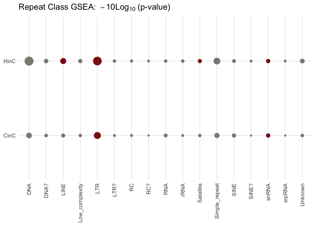
Figure 6.6: GSEA p-values in classes of repeat elements. The p-value deteremines whether the number of up-regulated repeat elements in the family is different from expected; the size of dots reflect the scaled p-values, -10log10(p-value); red dots present over-represented families (p-value < 0.1 and the number of up-regulated elements is higher than expected).
## quartz_off_screen
## 26.5 LTR retroelements distribution and activation
LTR retroelements were classified into ERV1, ERVL, ERVL-MaLR, Gypsy, others (non-classified ERV1?, ERVL?, Gypsy?, and LTR) families. ERVL-MaLR constitutes most of the LTR (44%), and next is ERVL (33%) and ERR1 (19%).
suppressPackageStartupMessages(library(plyranges))
percent <- function(prob) paste0(format(prob, digit=1), "%")
ltr <- canFam3.rmsk %>% plyranges::filter(repClass == "LTR") %>%
plyranges::mutate(repFamily=as.character(repFamily)) %>%
plyranges::mutate(repFamily=ifelse(repFamily %in% c("Gypsy?", "ERVL?", "ERV1?", "LTR"),
"Others", repFamily)) %>%
plyranges::mutate(rng_width = width(.)) %>%
plyranges::group_by(repFamily) %>%
plyranges::summarise(length = sum(rng_width)) %>% as.data.frame() %>%
dplyr::arrange(desc(length)) %>%
dplyr::mutate(prop = 100* (length/sum(length))) %>%
dplyr::mutate(ypos = cumsum(prop) - 0.5 * prop) %>%
dplyr::mutate(percent=percent(prop), label = paste0(repFamily, " (", percent, ")"))
# Basic piechart
ggplot(ltr, aes(x="", y=prop, fill=repFamily)) +
geom_bar(stat="identity", width=1, color="white", show.legend=FALSE) +
coord_polar("y", start=0) +
theme_void() +
geom_text(aes(y=ypos, x=c(1,1,1,1,1.2), label = label),
color = "white", size=4) +
scale_fill_brewer(palette="Set1")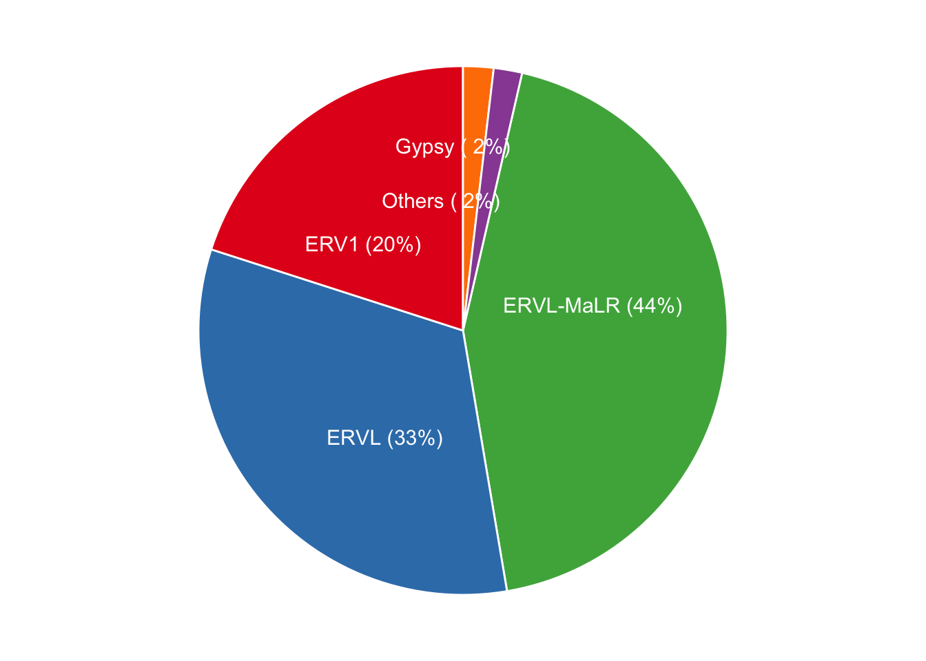
Figure 6.7: Distribution of LTR retroelement family. LTRs are categorized into ERV1, ERVL, ERVL-MaLR, Gypsy and ambibuguos, unclassified Others (ERVL?, Gypsy? ERVL1? and LTR) families. Almost 44% of LTRs belong to MaLR family in canFam3 genome.
LTR repeat family activation (ERV1, ERVL, MaLR) by violin plot: violin plot of LTR retroelements expression in each family; each dot represents a repeat element; red dots present up-regulated elements; diamond shape is the median expression of the family.
LTR <- comb %>% dplyr::filter(repClass_HinC == "LTR") %>%
dplyr::mutate(repFamily_HinC = factor(repFamily_HinC)) %>%
dplyr::select(repName, repFamily_HinC, repClass_HinC,
log2FoldChange_HinC, log2FoldChange_CinC, padj_HinC, padj_CinC) %>%
dplyr::rename(repFamily=repFamily_HinC, repClass=repClass_HinC) %>%
tidyr::gather(key="sample", value="log2FC", -repName, -repFamily, -repClass, -padj_HinC, -padj_CinC) %>%
dplyr::mutate(sample = ifelse(grepl("HinC", sample), "HinC", "CinC")) %>%
dplyr::mutate(padj = ifelse(sample == "HinC", padj_HinC, padj_CinC)) %>%
dplyr::mutate(DE_status = padj < 0.05) %>% # fix repFamily: put *? to others
dplyr::mutate(repFamily=as.character(repFamily)) %>%
dplyr::mutate(repFamily =
replace(repFamily, which(repFamily %in% c("ERV1?", "ERVL?", "Gypsy?", "LTR")), "Others"))
gg <- ggplot(LTR, aes(x=repFamily, y=log2FC)) +
#geom_boxplot(width=0.5, outlier.shape=NA) +
geom_violin(width=0.7) +
#geom_jitter(size=0.6, alpha=0.7, aes(color=DE_status), show.legend=FALSE) +
geom_dotplot(binaxis='y', stackdir='center', dotsize=0.5,
aes(color=DE_status, fill=DE_status),
alpha=0.9, show.legend=FALSE) +
stat_summary(fun.y=mean, geom="point", shape=23, size=2, color="red") +
theme_bw() +
facet_wrap( ~ sample, nrow=2) +
scale_fill_manual(values=c("ivory4", "firebrick4")) +
scale_color_manual(values=c("ivory4", "firebrick4")) +
labs(title="Repeat families in the LTR class", x="family")
gg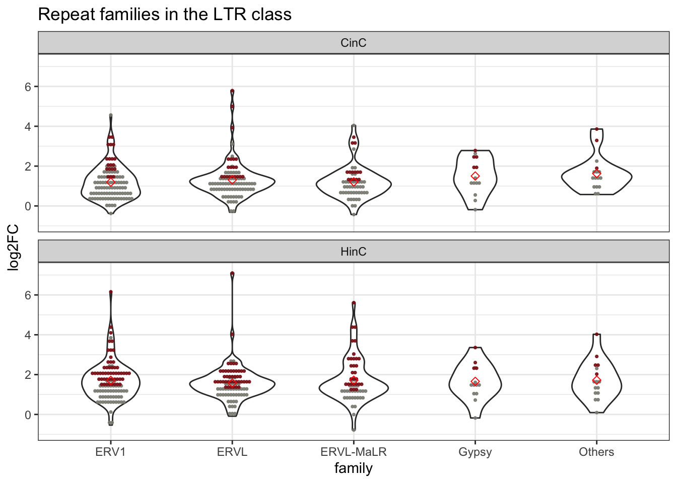
Figure 6.8: Violin plot of LTR retroelement expression in families of LTR. Each dot represents a repeat element; red dots present up-regulated elements; diamond shape is the median expression of the family.
## quartz_off_screen
## 2Frequency of up-regulated retroelements in LTR Family: DUX4 positively affects ~50% of retroelements in ERV1, ERVL and ERVL-MaLR families; DUXC affects 18% ~ 25% in these families.
freq <- LTR %>% group_by(sample, repFamily) %>%
summarise(n=dplyr::n(), n_up=sum(DE_status, na.rm=TRUE), prob=n_up/n)## `summarise()` regrouping output by 'sample' (override with `.groups` argument)ggplot(freq, aes(x=sample, y=prob, fill=repFamily) )+
geom_bar(stat="identity", show.legend=FALSE) +
facet_wrap( ~ repFamily, nrow=1) +
scale_fill_brewer(palette="Set1") +
geom_text(aes(label=format(prob, digit=2)), vjust=-0.3, size=3.5) +
theme_minimal()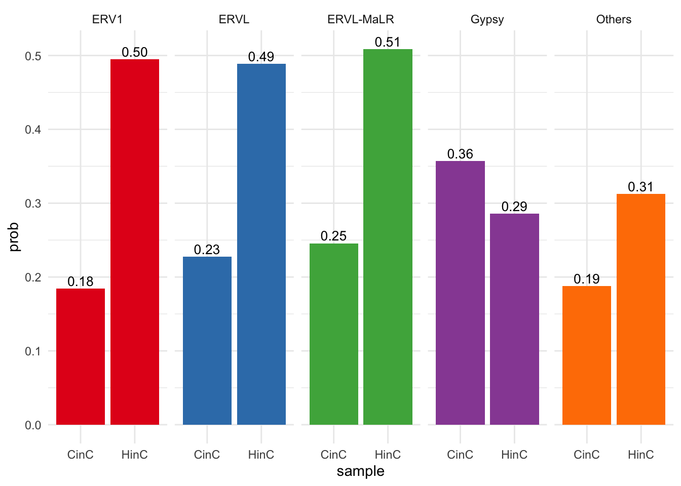
Figure 6.9: Percentage of activation of LTRs in each familiy.
6.6 Peaks distribution in class of repeat elements
The peaks distribution suggests that both DUX4 and DUXC enriched LTR subfamilies. Can we show that activating LTR leads to re-programing nearby gene’s structure, like we did at Whidden’s paper?
repeat class distribution in the canine geonome The code below considered the repeat class distribution on standard chromsomes in canFam3 genome.
# only keep the starndard chromosome
canFam3.rmsk <- keepStandardChromosomes(canFam3.rmsk, pruning.mode = "tidy",
species= "Canis_familiaris")
seq_info <- seqinfo(keepStandardChromosomes(TxDb.Cfamiliaris.UCSC.canFam3.ensGene))
genome_length <- sum(seqlengths(seq_info))
nonrepeat_length <- genome_length - sum(width(canFam3.rmsk))
repeat_class <- c("LTR", "SINE", "LINE", "DNA", "Simple_repeat")
canFam3.rmsk$instance_width <- width(canFam3.rmsk)
genome_repClass_freq <- canFam3.rmsk %>% plyranges::group_by(repClass) %>%
summarize(total_length = sum(instance_width)) %>% as.data.frame() %>%
dplyr::mutate(tidy_repClass = as.character(repClass)) %>%
dplyr::mutate(tidy_repClass = replace(tidy_repClass,
which(!tidy_repClass %in% repeat_class), "Other repeats")) %>%
tibble::add_row(repClass="Non-repetitive", total_length=nonrepeat_length,
tidy_repClass = "Non-repetitive") %>%
dplyr::mutate(tidy_repClass = factor(tidy_repClass,
levels=c(repeat_class, "Other repeats", "Non-repetitive"))) %>%
group_by(tidy_repClass) %>%
summarise(total_length = sum(total_length)) %>%
dplyr::mutate(frequency = total_length/genome_length * 100)## `summarise()` ungrouping output (override with `.groups` argument)## # A tibble: 7 x 3
## tidy_repClass total_length frequency
## <fct> <dbl> <dbl>
## 1 LTR 114911883 4.94
## 2 SINE 251299704 10.8
## 3 LINE 493299304 21.2
## 4 DNA 65806988 2.83
## 5 Simple_repeat 26825828 1.15
## 6 Other repeats 22743601 0.977
## 7 Non-repetitive 1352763403 58.1L1 and L2 distribution:
repeat_class <- c("LTR", "SINE", "LINE", "DNA", "Simple_repeat")
L1_family <- c("L1", "L2")
L1_family_freq <- canFam3.rmsk %>% plyranges::group_by(repFamily) %>%
summarize(total_length = sum(instance_width)) %>% as.data.frame() %>%
dplyr::filter(repFamily %in% c("L1", "L2")) %>%
dplyr::mutate(frequency = total_length/genome_length * 100)
L1_family_freq## repFamily total_length frequency
## 1 L1 398200270 17.107389
## 2 L2 82356072 3.538163L1_summary <- map(peaks_list, function(rng) {
total_peak <- length(rng)
df <- as(mcols(rng), "data.frame") %>% #tidy repClass
dplyr::mutate(l1_repFamily = as.character(repFamily)) %>%
dplyr::filter(l1_repFamily %in% c("L1", "L2")) %>%
group_by(l1_repFamily) %>%
dplyr::summarise(frequency = 100 * dplyr::n()/length(rng))
}) %>% bind_rows(.id="sample_name") %>%
dplyr::mutate(trans_factor = sapply(strsplit(sample_name, "_", fixed=TRUE), "[[", 3)) %>%
dplyr::mutate(clone_type = sapply(strsplit(sample_name, "_", fixed=TRUE), "[[", 4)) %>%
dplyr::mutate(Sample = paste0(trans_factor, "_", clone_type)) ## `summarise()` ungrouping output (override with `.groups` argument)
## `summarise()` ungrouping output (override with `.groups` argument)
## `summarise()` ungrouping output (override with `.groups` argument)
## `summarise()` ungrouping output (override with `.groups` argument)
## `summarise()` ungrouping output (override with `.groups` argument)Distribution of peaks in classes of repeat elements
repeat_class <- c("LTR", "SINE", "LINE", "DNA", "Simple_repeat", "Non-repetitive")
rep_summary <- map(peaks_list, function(rng) {
    total_peak <- length(rng)
    df <- as(mcols(rng), "data.frame") %>% #tidy repClass
      dplyr::mutate(tidy_repClass = as.character(repClass)) %>%
      dplyr::mutate(tidy_repClass = replace(tidy_repClass,
                                            which(is.na(tidy_repClass)),
                                            "Non-repetitive")) %>%
      dplyr::mutate(tidy_repClass = replace(tidy_repClass,
                                            which(!tidy_repClass %in% repeat_class), "Other repeats")) %>%
      dplyr::mutate(tidy_repClass = factor(tidy_repClass,
                                           levels=c(repeat_class[1:5],
                                                    "Other repeats",
                                                    "Non-repetitive"))) %>%
      group_by(tidy_repClass) %>%
      dplyr::summarise(frequency = 100 * dplyr::n()/length(rng))
}) %>% bind_rows(.id="sample_name") %>%
  dplyr::mutate(trans_factor = sapply(strsplit(sample_name, "_", fixed=TRUE), "[[", 3)) %>%
  dplyr::mutate(clone_type = sapply(strsplit(sample_name, "_", fixed=TRUE), "[[", 4)) %>%
  dplyr::mutate(Sample = paste0(trans_factor, "_", clone_type))

tidy_genome_repClass_freq <- genome_repClass_freq %>%
  add_column(sample_name = "whole_genome", .before="tidy_repClass") %>%
  dplyr::select(-total_length) %>%
  add_column(trans_factor = "none", clone_type="none", Sample="Genome")

re_name <-
  data.frame(Sample = c("Genome", "hDUX4_mono", "CCH_mono", "CALTh_poly"),
             re_Sample = c("Genome", "DUX4", "DUXC", "DUXC-ALT"))
## remove poly
rep_summary <- rep_summary %>% bind_rows(tidy_genome_repClass_freq) %>%
  dplyr::filter(!(Sample %in% c("hDUX4_poly", "CCH_poly"))) %>%
  dplyr::mutate(Sample=ifelse(Sample == "hDUX4_mono", "DUX4", Sample)) %>%
  dplyr::mutate(Sample=ifelse(Sample == "CCH_mono", "DUXC", Sample)) %>%
  dplyr::mutate(Sample=ifelse(Sample == "CALTh_poly", "DUXC-ALT", Sample)) %>%
  dplyr::mutate(Sample=factor(Sample,
                              levels = c("Genome","DUX4", "DUXC",
                                         "DUXC-ALT")))

col <- as.character(wes_palette(n=7, name="Darjeeling1", type="continuous"))

gg <- ggplot(rep_summary, aes(x=Sample, y=frequency, fill=tidy_repClass)) +
  geom_bar(stat="identity") +
  theme_minimal() +
  geom_text(aes(label=round(frequency)), position = position_stack(vjust = 0.5),
            color="gray10", size=3.5) +
  scale_fill_manual(values=col) +
  theme(axis.text.x = element_text(angle = 90, hjust = 1),
        axis.title.x = element_blank())   +
  labs(y="Frequency (%)", fill="Repeat class")
gg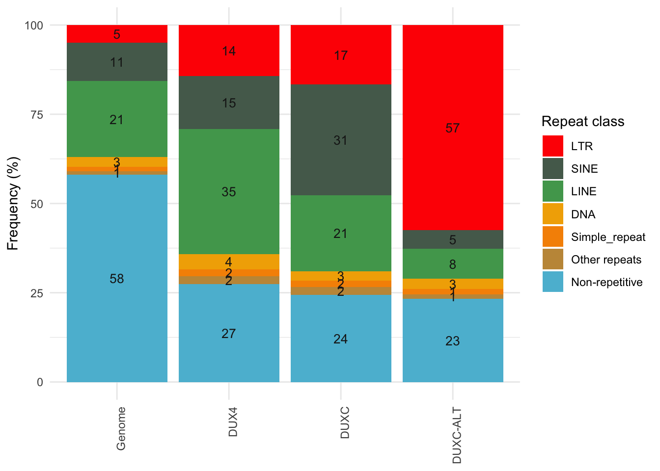
Figure 6.10: Distribution of peaks in classes of repeat elements.
# take out the polyclonal cell lines, except CALTh_poly
pdf(file.path(pkg_dir, "figures", "rmsk_peaks_repClass_freq_bar.pdf"), height=6, width=3.5)
gg
dev.off()
## quartz_off_screen
## 2# References
Peter G Hendrickson, Edward J Grow, Jessie A Doráis. 2017. “Conserved Roles of Mouse Dux and Human Dux4 in Activating Cleavage-Stage Genes and Mervl/Hervl Retrotransposons.” Nature Genetic, no. 6. https://doi.org/doi: 10.1038/ng.3844.