Quick Start

Quick Start for gimap

For more background on gimap and the calculations done here, read here

library(gimap)
#> Error in get(paste0(generic, ".", class), envir = get_method_env()) : 
#>   object 'type_sum.accel' not found

library(dplyr)
#> 
#> Attaching package: 'dplyr'
#> The following objects are masked from 'package:stats':
#> 
#>     filter, lag
#> The following objects are masked from 'package:base':
#> 
#>     intersect, setdiff, setequal, union

Set Up

First let’s create a folder we will save files to.

output_dir <- "output_timepoints"
dir.create(output_dir, showWarnings = FALSE)

example_data <- get_example_data("count")
#> Rows: 33170 Columns: 8
#> ── Column specification ────────────────────────────────────────────────────────
#> Delimiter: "\t"
#> chr (3): id, seq_1, seq_2
#> dbl (5): Day00_RepA, Day05_RepA, Day22_RepA, Day22_RepB, Day22_RepC
#> 
#> ℹ Use `spec()` to retrieve the full column specification for this data.
#> ℹ Specify the column types or set `show_col_types = FALSE` to quiet this message.

Setting up data

We’re going to set up three datasets that we will provide to the set_up() function to create a gimap dataset object.

• counts - the counts generated from pgPEN
• pg_ids - the IDs that correspond to the rows of the counts and specify the construct
• sample_metadata - metadata that describes the columns of the counts including their timepoints

counts <- example_data %>%
  select(c("Day00_RepA", "Day05_RepA", "Day22_RepA", "Day22_RepB", "Day22_RepC")) %>%
  as.matrix()

pg_id are just the unique IDs listed in the same order/sorted the same way as the count data.

pg_ids <- example_data %>%
  dplyr::select("id")

Sample metadata is the information that describes the samples and is sorted the same order as the columns in the count data.

sample_metadata <- data.frame(
  col_names = c("Day00_RepA", "Day05_RepA", "Day22_RepA", "Day22_RepB", "Day22_RepC"),
  day = as.numeric(c("0", "5", "22", "22", "22")),
  rep = as.factor(c("RepA", "RepA", "RepA", "RepB", "RepC"))
)

We’ll need to provide example_counts, pg_ids and sample_metadata to setup_data().

gimap_dataset <- setup_data(
  counts = counts,
  pg_ids = pg_ids,
  sample_metadata = sample_metadata
)

It’s ideal to run quality checks first. The run_qc() function will create a report we can look at to assess this.

run_qc(gimap_dataset,
       output_file = "example_qc_report.Rmd",
       overwrite = TRUE,
       quiet = TRUE)

You can take a look at an example QC report here.

gimap_dataset <- gimap_dataset %>%
  gimap_filter() %>%
  gimap_annotate(cell_line = "HELA") %>%
  gimap_normalize(
    timepoints = "day"
  ) %>%
  calc_gi()
#> Annotating Data
#> Rows: 1884 Columns: 3
#> ── Column specification ────────────────────────────────────────────────────────
#> Delimiter: ","
#> chr (3): gene, gene_symbol, entrez_id
#> 
#> ℹ Use `spec()` to retrieve the full column specification for this data.
#> ℹ Specify the column types or set `show_col_types = FALSE` to quiet this message.
#> Normalizing Log Fold Change
#> 
#> Calculating Genetic Interaction scores

Example output

Genetic interaction is calculated by:

• rep - indicates which sample from the original the data is from. Note the pretreatment is used for calculation and its statistics are not reported.
• pgRNA_target - what gene(s) were targeted by this the original pgRNAs for these data
• mean_expected_cs - the average expected genetic interaction score
• mean_gi_score - the average observer genetic interaction score
• target_type - describes whether the CRISPR design is targeting two genes (“gene_gene”), or a gene and a non targeting control (“gene_ctrl”) or a targeting control and a gene (“ctrl_gene”).
• p_val - p values from the testing whether a double knockout construct is significantly different in its genetic interaction score from single targets.
  
• fdr - False discovery rate corrected p values

gimap_dataset$gi_scores %>%
  dplyr::arrange(fdr) %>% 
  head() %>% 
  knitr::kable(format = "html") 

rep	pgRNA_target	mean_expected_cs	mean_observed_cs	mean_gi_score	target_type	p_val	fdr
Day22_RepA_late	NDEL1_NDE1	-1.8731292	-2.673450	-1.292412	gene_gene	0.0e+00	0.0000270
Day22_RepA_late	PFN2_PFN1	-1.5811362	-2.360606	-1.172104	gene_gene	1.0e-07	0.0000598
Day22_RepA_late	CNOT8_CNOT7	-0.2525986	-2.298083	-1.985598	gene_gene	9.0e-07	0.0003051
Day22_RepC_late	CNOT8_CNOT7	-0.6030327	-2.222123	-1.684182	gene_gene	4.0e-07	0.0004501
Day22_RepC_late	SHMT2_SHMT1	-1.0214662	-1.737076	-0.927188	gene_gene	9.0e-07	0.0004535
Day22_RepC_late	AKIRIN1_AKIRIN2	-1.7072333	-2.379270	-1.123690	gene_gene	5.9e-06	0.0006682

Plot the results

You can remove any samples from these plots by altering the reps_to_drop argument.

plot_exp_v_obs_scatter(gimap_dataset, reps_to_drop = "Day05_RepA_early")

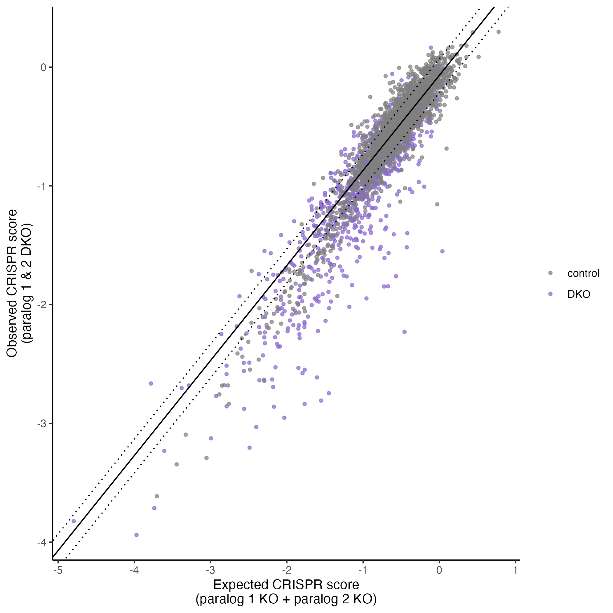
plot_rank_scatter(gimap_dataset, reps_to_drop = "Day05_RepA_early")

plot_volcano(gimap_dataset, reps_to_drop = "Day05_RepA_early", facet_rep = FALSE)

Here’s how you can save plots like the above.

ggplot2::ggsave("volcano_plot.png")
#> Saving 7.29 x 4.51 in image

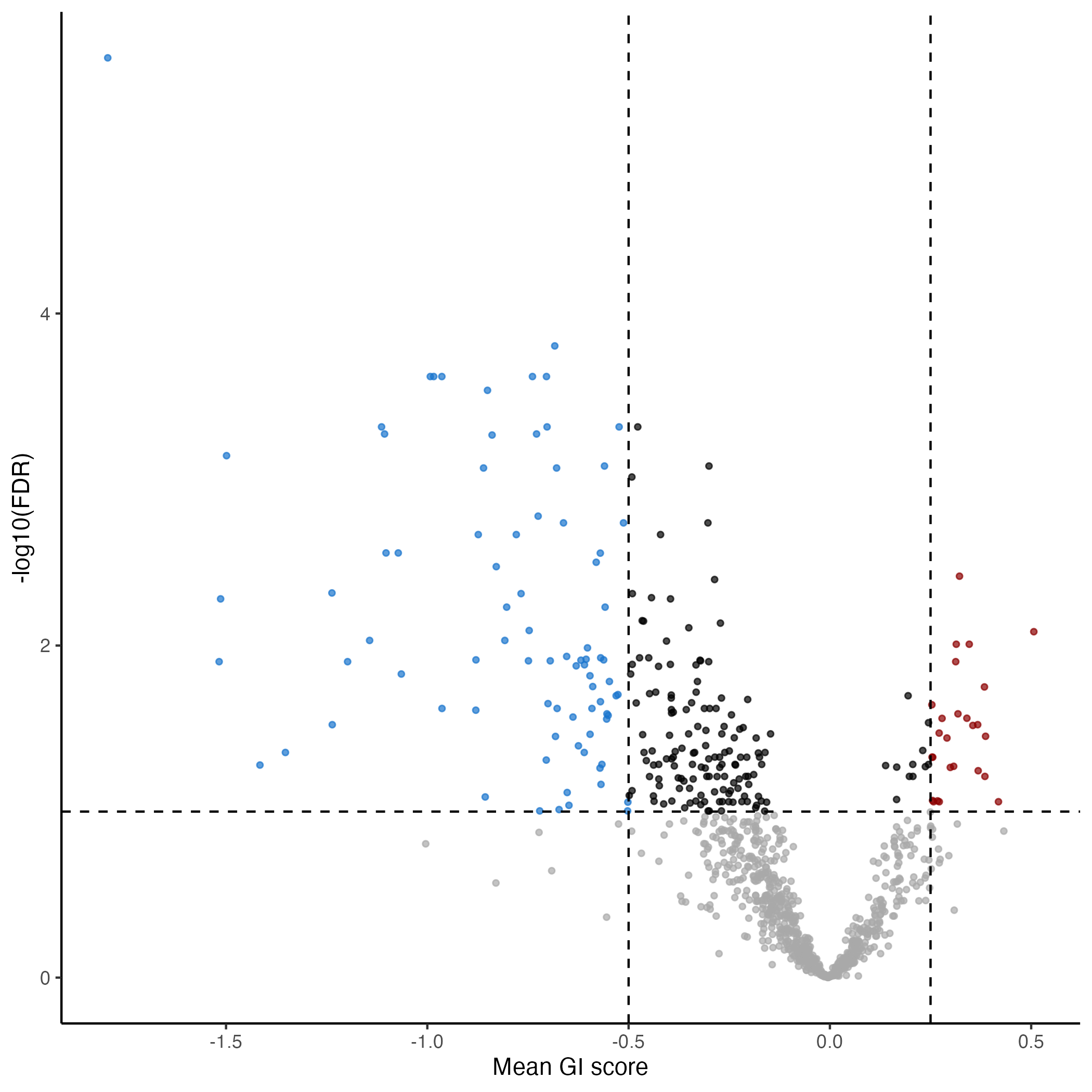
Plot specific target pair

We can pick out a specific pair to plot.

# "NDEL1_NDE1" is top result so let's plot that
plot_targets_bar(gimap_dataset, target1 = "NDEL1", target2 = "NDE1")

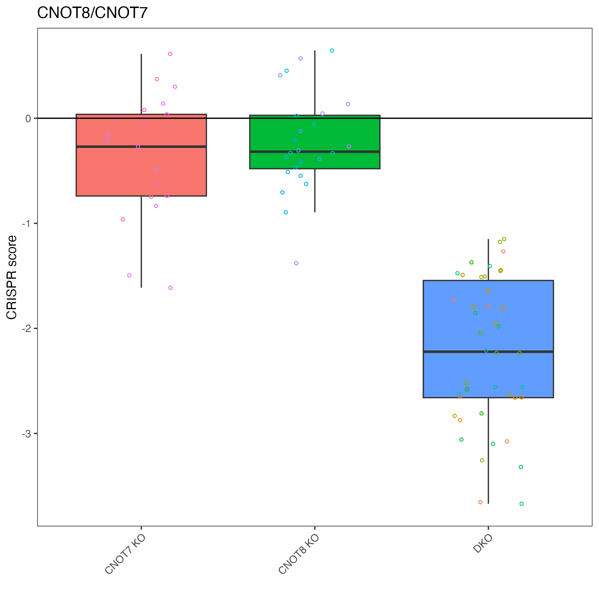
Saving data to a file

We can save all these data as an RDS or the genetic interaction scores themselves to a tsv file.

saveRDS(gimap_dataset, "gimap_dataset_final.RDS")

readr::write_tsv(gimap_dataset$gi_scores, "gi_scores.tsv")

Session Info

This is just for provenance purposes.

sessionInfo()
#> R version 4.4.0 (2024-04-24)
#> Platform: x86_64-apple-darwin20
#> Running under: macOS 15.1.1
#> 
#> Matrix products: default
#> BLAS:   /Library/Frameworks/R.framework/Versions/4.4-x86_64/Resources/lib/libRblas.0.dylib 
#> LAPACK: /Library/Frameworks/R.framework/Versions/4.4-x86_64/Resources/lib/libRlapack.dylib;  LAPACK version 3.12.0
#> 
#> locale:
#> [1] en_US.UTF-8/en_US.UTF-8/en_US.UTF-8/C/en_US.UTF-8/en_US.UTF-8
#> 
#> time zone: America/New_York
#> tzcode source: internal
#> 
#> attached base packages:
#> [1] stats     graphics  grDevices utils     datasets  methods   base     
#> 
#> other attached packages:
#> [1] dplyr_1.1.4 gimap_1.0.0
#> 
#> loaded via a namespace (and not attached):
#>  [1] sass_0.4.9         generics_0.1.3     tidyr_1.3.1        stringi_1.8.4     
#>  [5] hms_1.1.3          digest_0.6.37      magrittr_2.0.3     evaluate_1.0.1    
#>  [9] grid_4.4.0         timechange_0.3.0   RColorBrewer_1.1-3 fastmap_1.2.0     
#> [13] jsonlite_1.8.9     backports_1.5.0    purrr_1.0.2        scales_1.3.0      
#> [17] textshaping_0.4.1  jquerylib_0.1.4    cli_3.6.3          crayon_1.5.3      
#> [21] rlang_1.1.4        bit64_4.5.2        munsell_0.5.1      withr_3.0.2       
#> [25] cachem_1.1.0       yaml_2.3.10        parallel_4.4.0     tools_4.4.0       
#> [29] tzdb_0.4.0         colorspace_2.1-1   ggplot2_3.5.1      broom_1.0.7       
#> [33] curl_6.0.1         vctrs_0.6.5        R6_2.5.1           lifecycle_1.0.4   
#> [37] lubridate_1.9.4    snakecase_0.11.1   stringr_1.5.1      bit_4.5.0.1       
#> [41] fs_1.6.5           htmlwidgets_1.6.4  vroom_1.6.5        ragg_1.3.3        
#> [45] janitor_2.2.0      pkgconfig_2.0.3    desc_1.4.3         pkgdown_2.1.1     
#> [49] pillar_1.10.0      bslib_0.8.0.9000   gtable_0.3.6       glue_1.8.0        
#> [53] systemfonts_1.1.0  xfun_0.49          tibble_3.2.1       tidyselect_1.2.1  
#> [57] rstudioapi_0.17.1  knitr_1.49         farver_2.1.2       htmltools_0.5.8.1 
#> [61] labeling_0.4.3     rmarkdown_2.29     readr_2.1.5        pheatmap_1.0.12   
#> [65] compiler_4.4.0