gimap tutorial for treatments
gimap performs analysis of dual-targeting CRISPR screening data, with the goal of aiding the identification of genetic interactions (e.g. cooperativity, synthetic lethality) in models of disease and other biological contexts. gimap analyzes functional genomic data generated by the pgPEN (paired guide RNAs for genetic interaction mapping) approach, quantifying growth effects of single and paired gene knockouts upon application of a CRISPR library. A multitude of CRISPR screen types can be used for this analysis, with helpful descriptions found in this review (https://www.nature.com/articles/s43586-021-00093-4). Use of pgPEN and GI-mapping in a paired gRNA format can be found here (https://pubmed.ncbi.nlm.nih.gov/34469736/).
Requirements
Besides installing the gimap package, you will also need to install
wget if you do not already have it installed. This will allow you to
download the annotation files needed to run gimap.
To install this package you will need to run:
install.packages("gimap")Or you can install the development version from GitHub:
install.packages("remotes")
remotes::install_github("FredHutch/gimap")
Loading needed packages
library(dplyr)
output_dir <- "output_treatment"
dir.create(output_dir, showWarnings = FALSE)
Data loading and setup
In this example we are going to examine a dataset with drug treatments and controls.
Let’s examine this example pgPEN counts table. It’s divided into columns containing:
-
id: an ID corresponding to the names of paired guides -
seq_1: gRNA sequence 1, targeting “paralog A” -
seq_2: gRNA sequence 2, targeting “paralog B” -
pretreatment: The pretreated control -
dmsoA: Vehicle only for Replicate A -
dmsoB: Vehicle only for Replicate B -
drug1A: Drug treatment for Replicate A -
drug2B: Drug treatment for Replicate B
For the purposes of this tutorial, we can grab example data from the package.
example_data <- get_example_data("count_treatment")The metadata you have may vary slightly from this but you’ll want to make sure you have the essential variables and information regarding how you collected your data.
colnames(example_data)Setting up data
We’re going to set up three datasets that we will provide to the
set_up() function to create a gimap dataset
object.
-
counts- the counts generated from pgPEN -
pg_ids- the IDs that correspond to the rows of the counts and specify the construct -
sample_metadata- metadata that describes the columns of the counts including their timepoints
For this example we are using a treatment dataset where there is a pretreatment sample, two vehicle replicates and two drug treated replicates.
counts <- example_data %>%
  select(c("pretreatment", "dmsoA", "dmsoB", "drug1A", "drug1B")) %>%
  as.matrix()
The next datasets are metadata that describe the dimensions of the count data.
- These both need to be data frames.
- The sizes of these metadata must correspond to the dimensions of the counts data.
pg_id are just the unique IDs listed in the same
order/sorted the same way as the count data and can be used for mapping
between the count data and the metadata. This is required and very
important because it is necessary to know the IDs and be able to map
them to pgRNA constructs and counts data.
Sample metadata is the information that describes the samples and is sorted the same order as the columns in the count data.
You need to have two columns in the metadata you provide. You’ll need
to specify the names of these columns in the
gimap_annotate() function.
-
col_names- Must match the colnames of the counts data being submitted -
treatments- A factor variable that describes the treatments for these data. The label for the control specified in this column will need to be supplied to thegimap_normalize()function.
sample_metadata <- data.frame(
  col_names = c("pretreatment", "dmsoA", "dmsoB", "drug1A", "drug1B"),
  drug_treatment = as.factor(c("pretreatment", "dmso", "dmso", "drug", "drug"))
)
We’ll need to provide counts, pg_ids and
sample_metadata to setup_data().
Now let’s setup our data using setup_data(). Optionally
we can provide the metadata in this function as well so that it is
stored with the data.
gimap_dataset <- setup_data(
  counts = counts,
  pg_ids = pg_ids,
  sample_metadata = sample_metadata
)
You’ll notice that this set up gives us a list of formatted data.
This contains the original counts we gave setup_data()
function but also normalized counts, and the total counts per
sample.
-
raw_counts: The original counts data that illustrates the number of cells alive in the sample. This data has samples as the columns and the paired guide constructs as rows. -
counts_per_sample: Add up all the counts for each sample over all of the paired guide designs. - Transformed data: This section contains the various types of normalized and adjusted data made from the raw counts data.
-
count_norm- For each sample, the data is normalized-log10(( counts +1) / total counts for the sample over all the pg designs )) -
cpm- For each sample this is calculated by taking thecounts / total counts for the sample over all the pg designs)*1e6 -
log2cpm: log-2 transformed counts per million this is calculated bylog2(cpms + 1) - pg_metadata: paired guide metadata - information that describes the paired-guided RNA designs. This may include the sequences used in the CRISPR design as well as what genes are targeted.
-
sample_metadata: Metadata that describes the samples. This likely includes the time point information, replicates, sample IDs, and any other additional information that is needed regarding the experimental setup.
str(gimap_dataset)Let’s see how many rows of data we have.
nrow(gimap_dataset$transformed_data$log2_cpm)Quality Checks
The first step is running some quality checks on our data. The
run_qc() function will create a report we can look at to
assess this.
The report includes several visualizations of raw/unfiltered data:
- distribution of normalized counts for each sample. The goal of determining this distribution is to identify pgRNA counts that are low at the start of the screen - before any type of phenotypic or growth selection is occurring, either in the T0 or plasmid sample. These low abundance pgRNAs should be removed from the analysis. [the goal section here doesn’t fit my expectations/understanding of this plot.]
- histogram of
log2cpmvalues for each individual sample: this helps users identify samples that do not have a normal distribution of reads and inform the upcoming filtering steps. - sample correlation heatmap: generates a heatmap using cpm values for each replicate/sample. This heatmap gives an overview on how similar samples are. Replicates should correlate well, and cluster together, while each timepoint sample should be different from the T0. This analysis will also allow users to identify potential sample swaps, if correlation scores between replicates is poor.
- A histogram that shows the variance within replicates for each pgRNA construct. For each pgRNA construct, the variance among the 3 replicates is found and a distribution is constructed by looking at these variances together.
- A histogram of the log2 CPM values of pgRNA constructs at the plasmid time point. This graph relates to a plasmid filter that can be applied to the data, but the plot displays all of the data prior to a filter being applied.
This report also includes several visualizations after filters are applied:
There is a filter that flags pgRNA constructs where any of the time points have a count of zero. - We include a bar plot that shows the number of pgRNA constructs which have counts of zero in either 0, 1, 2, or 3 replicates. - We include a table that specifies how many pgRNAs would be filtered out by applying this filter.
There is a filter that flags pgRNA constructs that have low log2 CPM counts for the day 0 or plasmid time point. - The histogram of the log2 CPM values of pgRNA constructs at the plasmid time point mentioned earlier does have a dashed line specifying the lower outlier (or a user defined cutoff) and pgRNA constructs with a plasmid log2 CPM lower than that value can be filtered out. - We include a table that specifies how many pgRNAs would be filtered out by applying this filter.
There is a filter that flags pgRNA constructs that have low log2 CPM counts for the day 0 or plasmid time point. - The histogram of the log2 CPM values of pgRNA constructs at the plasmid time point mentioned earlier does have a dashed line specifying the lower outlier (or a user defined cutoff) and pgRNA constructs with a plasmid log2 CPM lower than that value can be filtered out. - We include a table that specifies how many pgRNAs would be filtered out by applying this filter.
run_qc(gimap_dataset,
  output_file = file.path(output_dir, "example_qc_report.Rmd"),
  overwrite = TRUE,
  quiet = TRUE
)
You can take a look at an example QC report here.
Filtering the data
After considering the QC report and which filters are
appropriate/desired for your data, you can apply filters to the data
using the gimap_filter function.
gimap_filtered <- gimap_dataset %>%
  gimap_filter()
How many rows of data do we have now after filtering?
nrow(gimap_filtered$filtered_data$transformed_log2_cpm)
str(gimap_filtered$filtered_data)Let’s take a look at how many rows of data we have left:
nrow(gimap_filtered$filtered_data$transformed_log2_cpm)As you can see from the output above, there are fewer pgRNA constructs in the filtered dataset following completion of filtering.
The filtering step also stores two tables of information that you may want to use or report.
-
$filtered_data$removed_pg_idsis a table that has the pgRNA construct IDs that are removed following completion of filtering in theidcolumn and the relevant filter(s) that led to removal as a comma separated list in therelevantFilterscolumn -
$filtered_data$all_reps_zerocount_idsis a table that lists the IDs of pgRNA constructs which had a count of 0 for all final timepoint replicates. These pgRNA constructs are NOT necessarily filtered out
Now that you’ve performed QC and filtering, the rest of the pipeline can be run
- First annotating the data set (expression levels, copy number, etc.)
with DepMap data. For the annotation step, you must specify
which
cell_lineyour data uses so that the correct corresponding DepMap data is used for annotation. This function isgimap_annotate() - Then the data is normalized with the
gimap_normalize()function.timepointsneeds to be specified pointing to the correct column names from thesample_datapassed to thesetup_data()function earlier. - Genetic interaction scores are computed with the
calc_gi()function.
Normalization and calculating scores
gimap_dataset <- gimap_filtered %>%
  gimap_annotate(cell_line = "PC9") %>%
  # Whatever is specified for "control_name" is what will be used to normalize other data points
  gimap_normalize(
    treatments = "drug_treatment",
    control_name = "pretreatment"
  ) %>%
  calc_gi()
Here’s what’s included in the GI Scores table:
head(gimap_dataset$gi_scores)Let’s check out the top results
Plot the results
You can remove any samples from these plots by altering the
reps_to_drop argument.
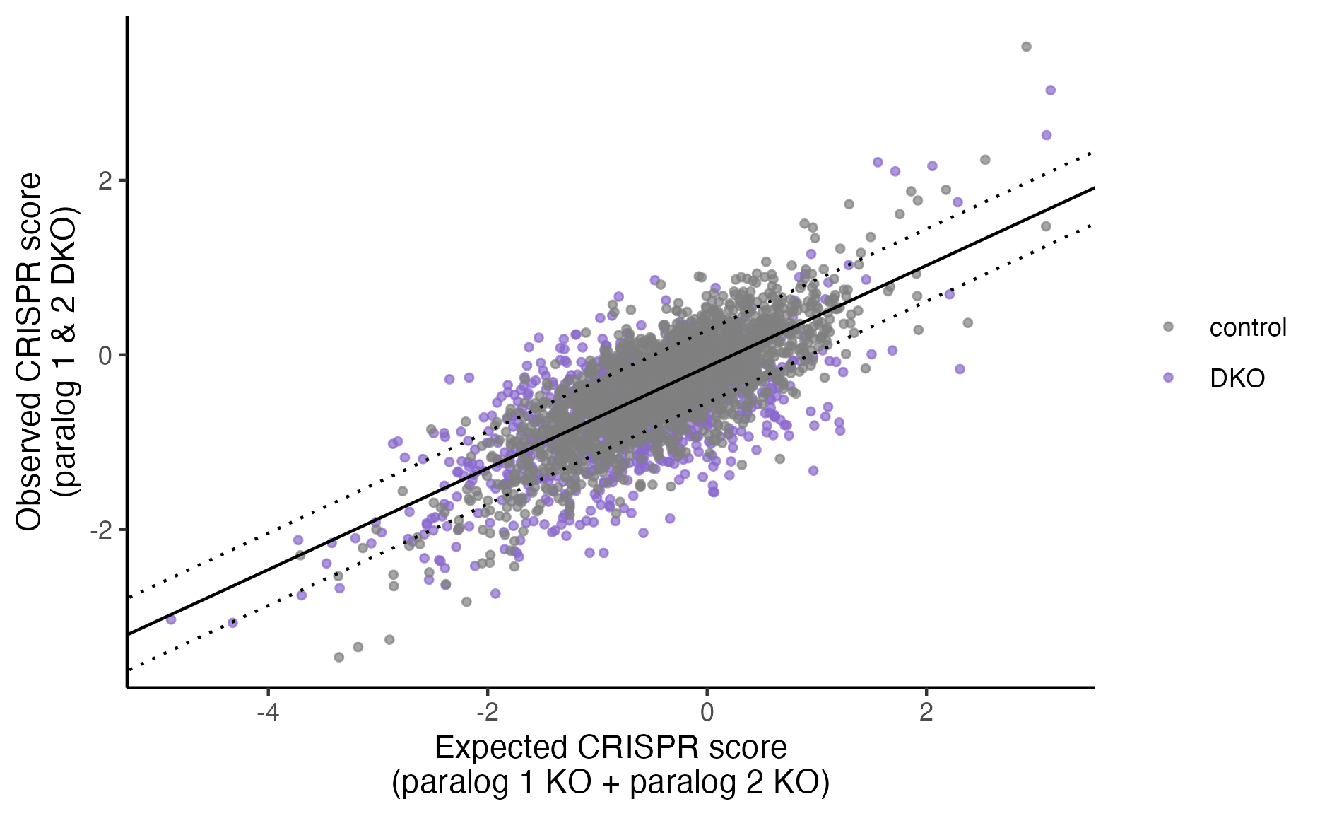
plot_exp_v_obs_scatter(gimap_dataset)

# Save it to a file
ggsave(file.path(output_dir, "exp_v_obs_scatter.png"))
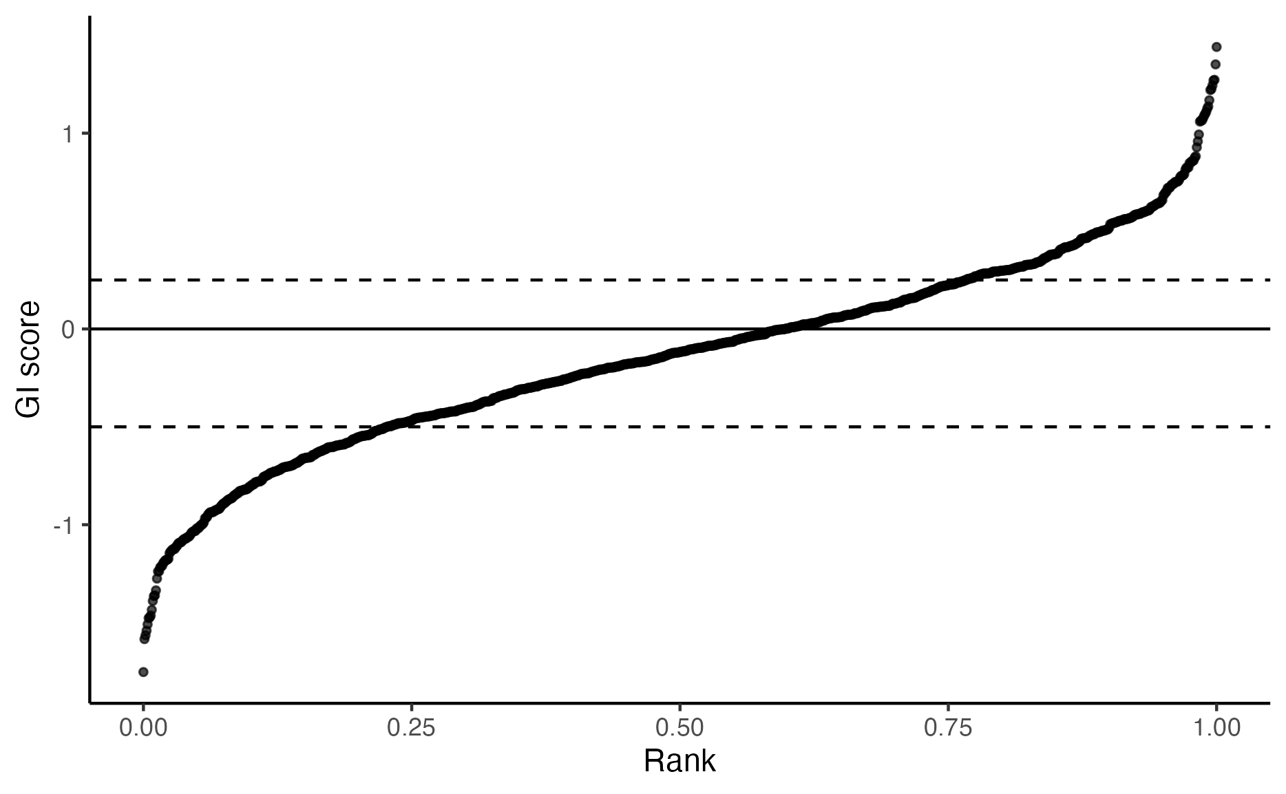
plot_rank_scatter(gimap_dataset)

# Save it to a file
ggsave(file.path(output_dir, "plot_rank_scatter.png"))
plot_volcano(gimap_dataset)

# Save it to a file
ggsave(file.path(output_dir, "volcano_plot.png"))
Plot specific target pair
We can pick out a specific pair to plot.
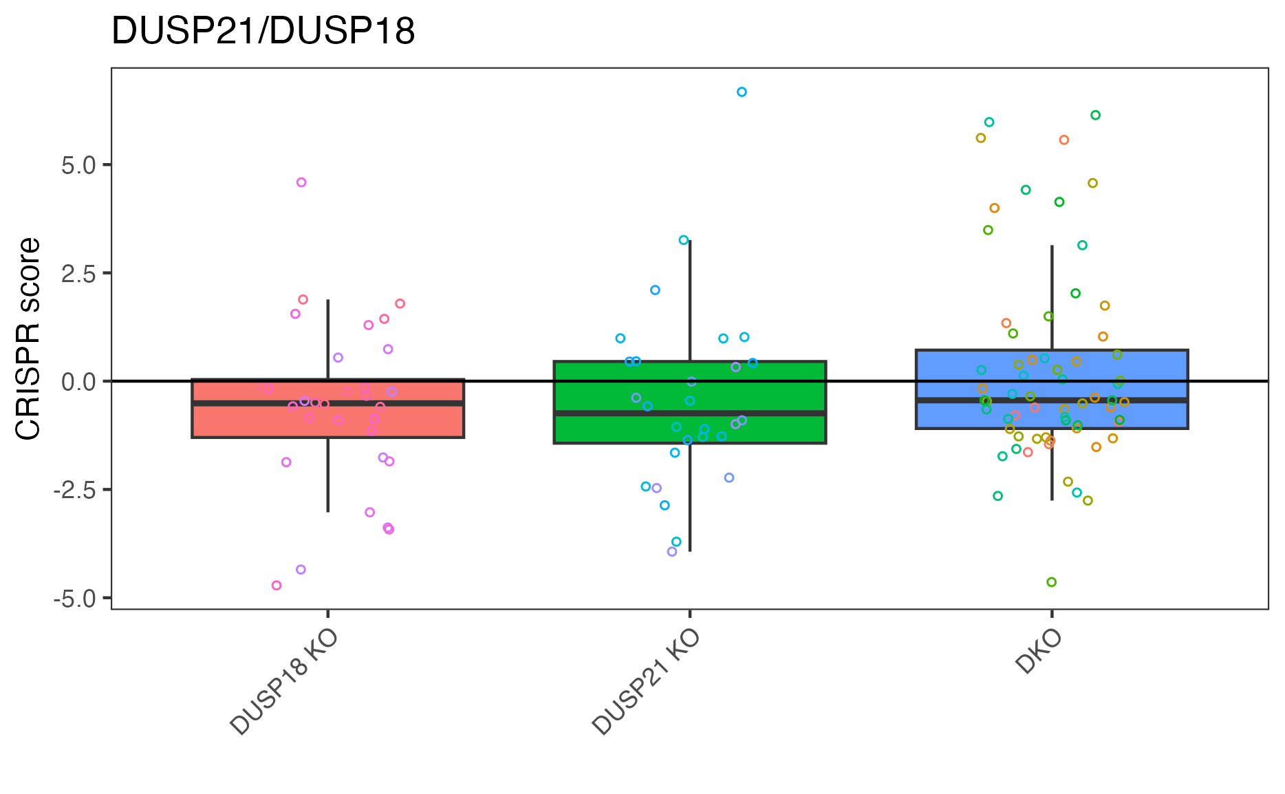
# "DUSP21_DUSP18" is top result so let's plot that
plot_targets(gimap_dataset, target1 = "DUSP21", target2 = "DUSP18")

# Save it to a file
ggsave(file.path(output_dir, "DUSP21_DUSP18.png"))
Saving results to files
We can save the genetic interactions scores like this:
We can save all these data as an RDS.
Session Info
This is just for provenance purposes.
sessionInfo()
#> R version 4.4.0 (2024-04-24)
#> Platform: x86_64-apple-darwin20
#> Running under: macOS 15.3.2
#>
#> Matrix products: default
#> BLAS:   /Library/Frameworks/R.framework/Versions/4.4-x86_64/Resources/lib/libRblas.0.dylib
#> LAPACK: /Library/Frameworks/R.framework/Versions/4.4-x86_64/Resources/lib/libRlapack.dylib;  LAPACK version 3.12.0
#>
#> locale:
#> [1] en_US.UTF-8/en_US.UTF-8/en_US.UTF-8/C/en_US.UTF-8/en_US.UTF-8
#>
#> time zone: America/New_York
#> tzcode source: internal
#>
#> attached base packages:
#> [1] stats     graphics  grDevices utils     datasets  methods   base
#>
#> other attached packages:
#> [1] gimap_1.0.3
#>
#> loaded via a namespace (and not attached):
#>  [1] gtable_0.3.6       jsonlite_1.8.9     dplyr_1.1.4        compiler_4.4.0
#>  [5] tidyselect_1.2.1   stringr_1.5.1      snakecase_0.11.1   tidyr_1.3.1
#>  [9] jquerylib_0.1.4    systemfonts_1.2.1  scales_1.3.0       textshaping_1.0.0
#> [13] yaml_2.3.10        fastmap_1.2.0      ggplot2_3.5.1      R6_2.5.1
#> [17] generics_0.1.3     knitr_1.49         htmlwidgets_1.6.4  tibble_3.2.1
#> [21] janitor_2.2.1      desc_1.4.3         openssl_2.3.2      munsell_0.5.1
#> [25] lubridate_1.9.4    RColorBrewer_1.1-3 bslib_0.8.0.9000   pillar_1.10.1
#> [29] rlang_1.1.5        stringi_1.8.4      cachem_1.1.0       xfun_0.50
#> [33] fs_1.6.5           sass_0.4.9         timechange_0.3.0   cli_3.6.3
#> [37] pkgdown_2.1.1      magrittr_2.0.3     digest_0.6.37      grid_4.4.0
#> [41] rstudioapi_0.17.1  askpass_1.2.1      lifecycle_1.0.4    vctrs_0.6.5
#> [45] pheatmap_1.0.12    evaluate_1.0.3     glue_1.8.0         ragg_1.3.3
#> [49] colorspace_2.1-1   purrr_1.0.4        rmarkdown_2.29     httr_1.4.7
#> [53] tools_4.4.0        pkgconfig_2.0.3    htmltools_0.5.8.1