7 Bilateral comparison

# load libraries
suppressPackageStartupMessages(library(tidyverse))
suppressPackageStartupMessages(library(DESeq2))
suppressPackageStartupMessages(library(writexl))
suppressPackageStartupMessages(library(knitr))
suppressPackageStartupMessages(library(kableExtra))
# parameters and load data sets
pkg_dir <- "/Users/cwon2/CompBio/Wellstone_BiLateral_Biopsy"
draft_fig_dir <- file.path(pkg_dir, "manuscript", "figures")
load(file.path(pkg_dir, "data", "comprehensive_df.rda"))
load(file.path(pkg_dir, "data", "dds.rda"))
load(file.path(pkg_dir, "data", "all_baskets.rda"))

# tidy annotation 
anno_gencode35 <- as.data.frame(rowData(dds)) %>%
  rownames_to_column(var="gene_id") %>% #BiLat study using Gencode 35
  dplyr::mutate(ens_id=str_replace(gene_id, "\\..*", ""))
# tidy column data
col_data <- as.data.frame(colData(dds)) %>%
  dplyr::mutate(sample_id = str_replace(sample_name, "[b]*_.*", "")) 

7.1 Random pairing simulation to show symmetric trends on MRI characteristics

Of 34 subjects, ten were rated STIR+ in both TAs, 19 STIR- bilaterally, and only five discordant for STIR. Our question was, given 43- STIR and 25 STIR+ to form 34 pairs, what are the expected values of the STIR+, STIR- and discordant STIR-/STIR+ pairs? Are the observed values different from the expected values?

To answer the question, we performed 1000 runs of simulation, in which each run, 34 pairs were randomly drowned from 43 STIR- and 25 STIR+ samples, yielding the numbers of STIR+, STIR-, and discordance STIR+/- pairs. This simulation built three distributions of the number of three types of pairs, and the expected values of each pair type are 4.5 pairs for STIR+, 13.5 for STIR- and 16 and STIR+/-. The observed values of STIR+ (10) and STIR- (19) pairs reveal symmetric trends in STIR characteristics.

# simulation distribution of the STIR+/+ (1,1), STIR-/- (0,0), and STIR-/+ (0,1) paire # 0 = STIR-
# 1 = STIR+
n_simulation <- 10000
sim_list <- vector("list", n_simulation)
for (j in 1:n_simulation) {
  n_pos <- 25 # 1: STIR+
  n_neg <- 43 # 0: STIR-
  n_pairs <- (n_pos + n_neg) / 2

  set.seed <- j
 
  res <- vector("integer", n_pairs)
  for (i in 1:n_pairs) {
    stir <- c(rep(1, n_pos), rep(0, n_neg))
    res[i] <- sum(sample(x=stir, 2, replace=FALSE))
    n_pos <- n_pos - res[i]
    n_neg <- n_neg - (2-res[i])
  }

  sim_list[[j]] <- table(res)
}

sim_res <- do.call(rbind, sim_list) %>%
  as.data.frame() %>%
  rename(`STIR-/-`= `0`, `STIR+/-`=`1`, `STIR+/+`=`2`) %>%
  gather(key="pairs", value="n")

annot <- sim_res %>% group_by(pairs) %>%
  summarise(mu = mean(n)) %>%
  dplyr::mutate(x_mu = mu, y_mu = 0) %>%
  dplyr::mutate(x_n=c(19, 5, 10), y_n=0) %>%
  dplyr::mutate(mu_label = format(mu, digit=2))

ggplot(sim_res, aes(x=n)) +
   geom_density(adjust=3.5, n=256) +
   #geom_histogram(bins=10) +
   facet_wrap( ~ pairs, nrow=3) +
   geom_point(data=annot, aes(x=x_n, y=y_n), 
              size=2, color="red", shape=4) +
   geom_text(data=annot, aes(x=x_mu, y=y_mu, 
                             label=paste0("mu = ", mu_label)), 
             hjust=0, vjust=0, color="gray50") +
   geom_vline(data=annot, aes(xintercept=mu),
              linetype="dashed", color="gray50") +
   labs(x="number of pairs", y="density") +
   theme_bw()
ggsave(file.path(pkg_dir, "figures", "STIR-2000-simulation-pairs.pdf"), 
       width=4, height=4)   
}

7.2 Fat infiltration

The Pearson correlation between right and left fat infiltration is 0.82.

fat_cor <- comprehensive_df %>% 
  dplyr::select(Subject, location, Fat_Infilt_Percent) %>%
  spread(key=location, value=Fat_Infilt_Percent) %>%
  drop_na(L, R) %>%
  summarise(cor=cor(L, R))
fat_cor
#> # A tibble: 1 × 1
#>     cor
#>   <dbl>
#> 1 0.821

comprehensive_df %>% 
  dplyr::select(Subject, location, Fat_Infilt_Percent) %>%
  spread(key=location, value=Fat_Infilt_Percent) %>%
  drop_na(L, R)  %>%
  ggplot(aes(x=L, y=R)) +
    geom_point(size=1) +
    geom_smooth(method="lm", se=FALSE, 
                color="grey75", alpha=0.3, linewidth=0.7) +
    #geom_abline(slope=1, intercept=0, color="grey50",
    #           linetype="dashed", alpha=0.5) +
    theme_minimal() +
    labs(title="Whole muscle fat percent", x="Left", y="Right") +
    theme(plot.title = element_text(hjust = 0.5, size=10),
          panel.grid.minor = element_blank(),
          axis.title = element_text(size=8)) +
    annotate("text", x=Inf, y=-Inf, color="gray25",
             size=3, hjust=1, vjust=-2,
             label=paste0("Pearson=", format(fat_cor$cor[1],
                                             digit=2)))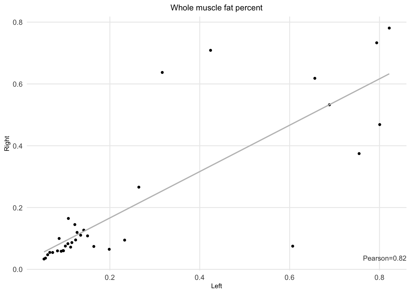 

Figure 7.1: Left and right whole muscle fat percent.

ggsave(file=file.path(draft_fig_dir,
                      "fat-infilt-left-and-right.pdf"),
       width=2.5, height=2)

7.3 Muscle strength

data <- comprehensive_df %>% 
  dplyr::select(Subject, location, `Foot Dorsiflexors`) %>%
  spread(key=location, value=`Foot Dorsiflexors`) %>%
  drop_na(L, R) 

strength_cor <- data %>% summarise(cor=cor(L, R))

ggplot(data, aes(x=L, y=R)) +
    geom_point(size=1) +
    geom_smooth(method="lm", se=FALSE, 
                color="grey75", alpha=0.3, linewidth=0.7) +
    #geom_abline(slope=1, intercept=0, color="grey50",
    #            linetype="dashed", alpha=0.5) +
    theme_minimal() +
    labs(title="Foot Dorsiflexors", x="Left", y="Right") +
    theme(plot.title = element_text(hjust = 0.5, size=10),
          panel.grid.minor = element_blank(),
          axis.title = element_text(size=8)) +
    annotate("text", x=Inf, y=-Inf, color="gray25",
             size=3, hjust=1, vjust=-2,
             label=paste0("Pearson=", format(strength_cor$cor[1],
                                             digit=2)))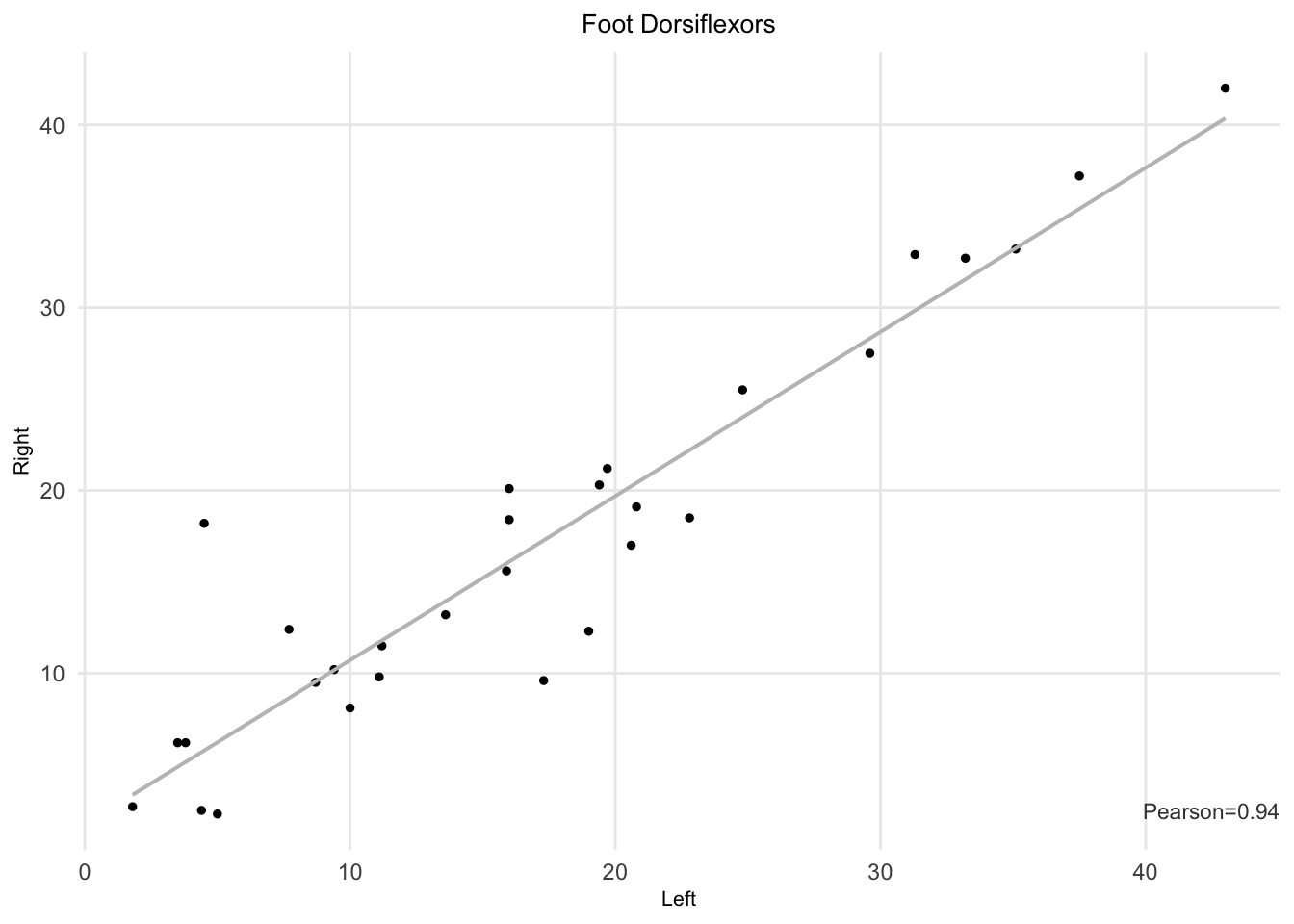 

Figure 7.2: Left and right TA muscle strength (foot dorsiflexors).

ggsave(file=file.path(draft_fig_dir,
                      "dorsiflexors-infilt-left-and-right.pdf"),
       width=2.5, height=2)

7.4 Histopathological variables

data <- comprehensive_df %>% 
  dplyr::select(Subject, location, `Cumulative Score`,
                `I. Variability in Fiber`,
                `II. Extent of Central Nucleation`,
                `III. Necrosis/Regeneration`,
                `IV. Interstitial Fiobrsis`) %>%
  dplyr::rename(`histopathological score`=`Cumulative Score`,
         `Variability in Fiber` = `I. Variability in Fiber`,
         `Extent of Central Nucleation` = `II. Extent of Central Nucleation`,
         `Necrosis/Regeneration`=`III. Necrosis/Regeneration`,
         `Interstitial Fiobrsis`=`IV. Interstitial Fiobrsis`) %>%
  gather(key=pathology_var, value=scores, -Subject, -location) %>%
  spread(key=location, value=scores) %>%
  drop_na(L, R) %>%
  dplyr::mutate(
    pathology_var=factor(pathology_var, 
                         levels=c("Variability in Fiber",
                                  "Extent of Central Nucleation",
                                  "Necrosis/Regeneration",
                                  "Interstitial Fiobrsis",
                                  "histopathological score")))
                                  #"STIR_RATING",
                                  #"FAT_FRACTION", 
                                  #"Fat_Infilt_Percent",
                                  #"Foot Dorsiflexors")))

path_cor <- data %>% group_by(pathology_var) %>%
  summarise(cor=cor(L, R)) 
  

ggplot(data, aes(x=L, y=R)) +
  geom_jitter(width=0.1, height=0.1, size=1) +
    geom_smooth(method="lm", se=FALSE) +
    geom_abline(slope=1, intercept=0, color="grey50",
                linetype="dashed", alpha=0.5) +
    theme_classic() +
    facet_wrap(~pathology_var, scale="free") +
    labs(title="Pathological scores bilateral correlation (Pearson)",
         x="Left", y="Right") +
    theme(plot.title = element_text(hjust = 0.5, size=12),
          axis.title = element_text(size=10)) +
    geom_text(data=path_cor, aes(label=format(cor, digit=2)),
              x=Inf, y=-Inf, color="gray25", 
              hjust=1, vjust=-1.5)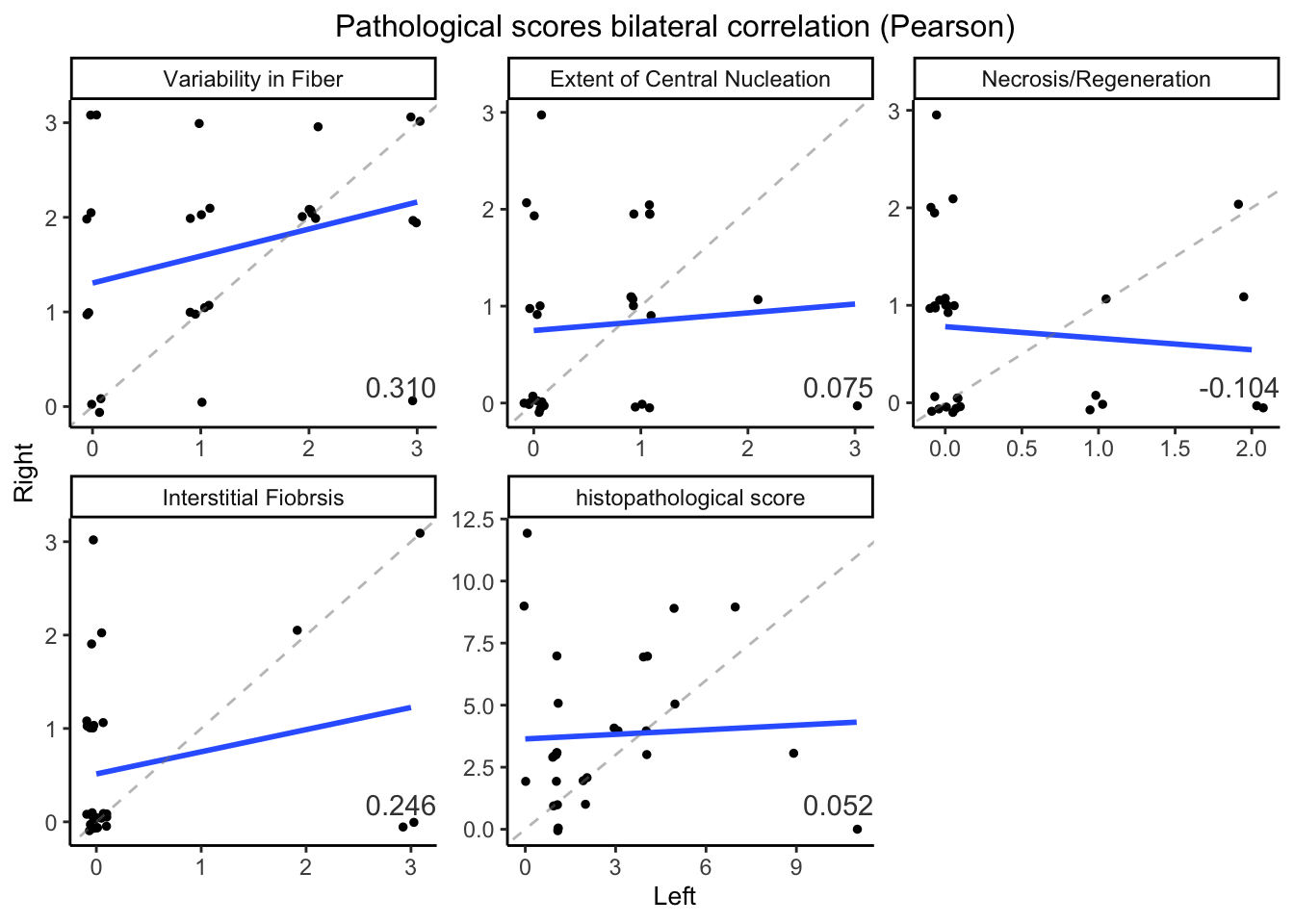

Figure 7.3: Lift and right TA muscle histopathological variables.

ggsave(file.path(draft_fig_dir, "bilateral_cor_pathological_var.pdf"), width=6, height=4)    

7.5 FSHD-signatures bilateral comparisons

7.5.1 Per-gene correlation

We calculated the left-t-right correlation for every genes in the baskets. The expression level used here is TPM.

# get TPM for each gene
bilat_tpm <- map_dfr(names(all_baskets), function(basket_name) {
    id <- all_baskets[[basket_name]]$gencode_v35
    tpm <- assays(dds[id])[["TPM"]] %>% t(.) %>% 
      as.data.frame() %>%
      rownames_to_column(var="sample_id") %>%
      dplyr::mutate(sample_id = str_replace(sample_id, 
                                            "[b]*_.*", "")) %>%
      gather(key=gene_id, value=TPM, -sample_id) %>% 
      left_join(anno_gencode35, by="gene_id") %>%
      dplyr::select(-ens_id, -gene_id, -gene_type) %>%
      left_join(dplyr::select(col_data, sample_id, location,
                              Subject), by="sample_id") %>%
      dplyr::select(-sample_id) %>%
      spread(key=location, value=TPM) %>% 
      drop_na(L, R) %>%
      dplyr::mutate(basket=basket_name)
}) %>% 
  dplyr::mutate(basket=factor(basket, levels=names(all_baskets))) 
#  dplyr::filter(!Subject %in% c("13-0007", "13-0009"))

gene_cor <- bilat_tpm %>% 
  drop_na(L, R) %>%
  dplyr::mutate(L_log = log10(L+1), R_log=log10(R+1)) %>%
  group_by(basket, gene_name) %>% 
  summarise(correlation=cor(L, R), cor_log = cor(L_log, R_log)) 

cor_mean <- gene_cor %>% 
  drop_na(correlation, cor_log) %>% 
  dplyr::filter(!basket %in% c("DUX4-M", "DUX4-M12")) %>%
  group_by(basket) %>%
  summarise(cor_mean = mean(correlation))
knitr::kable(cor_mean, caption="Mean of correlation of genes in each baskets calculated by TPM on L/R muscle.")

Table 7.1: Mean of correlation of genes in each baskets calculated by TPM on L/R muscle.

basket	cor_mean
DUX4-M6	0.6521460
ECM	0.5126943
Inflamm	0.4809635
Complement	0.6574381
IG	0.8281996

gene_cor %>% drop_na(correlation) %>%
  dplyr::filter(!basket %in% c("DUX4-M", "DUX4-M12")) %>%
  ggplot(aes(x=basket, y=correlation)) +
    geom_boxplot(width=0.5, outlier.shape=NA) +
    geom_point(alpha=0.6, size=2, color="grey50") +
    stat_summary(fun=mean, geom="point", shape=5, size=2.5,  
                 alpha=0.6, fill="red") +
    #geom_point(data=cor_mean, color="red", alpha=0.6) +
    theme_minimal() +
    labs(x="", y="Bilateral correlation (Pearson)") +
    theme(axis.title=element_text(size=10), 
          axis.text.x = element_text(angle = 90, 
                                     vjust = 0.5, hjust=1))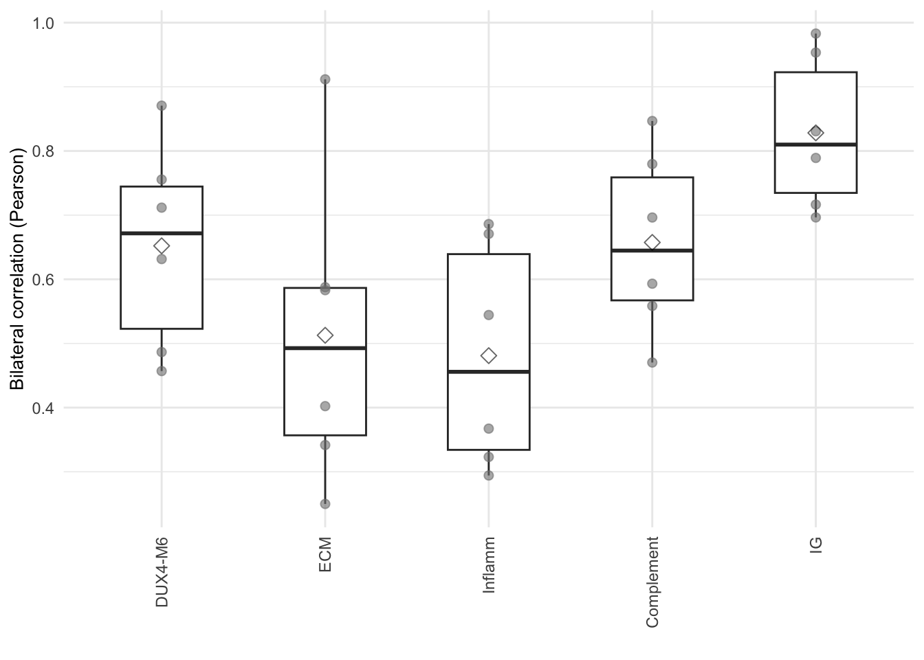

ggsave(file=file.path(draft_fig_dir,
                      "bilat-basket-comparison-cor-by-gene.pdf"),
       width=2, height=3)  

Scatter plot for each genes 6 by 5 scatter plots

dux4_corr <- gene_cor %>% dplyr::filter(basket == "DUX4-M6") %>%
  dplyr::mutate(formated=format(correlation, digit=2))

bilat_tpm %>% dplyr::filter(basket %in% c("DUX4-M6")) %>%
  ggplot(aes(x=L, y=R)) +
    geom_point(size=1, alpha=0.7) +
    geom_smooth(method="lm", linewidth=0.5, se=FALSE, alpha=0.5) +
    facet_wrap(~gene_name, scales="free", nrow=1) +
    geom_text(data=dux4_corr, aes(label=paste0("r=", formated)),
              x=Inf, y=-Inf, color="gray25", 
              hjust=1, vjust=-1, size=2.5) +
    theme_classic() +
    theme(plot.title=element_text(hjust=0.5, size=10)) +
    labs(x="left", y="right", title="DUX4-M6") +
    scale_y_continuous(trans="log10") + 
    scale_x_continuous(trans="log10") 

ggsave(file.path(draft_fig_dir, "bilateral_cor_DUX4_basket_genes.pdf"),
       width=7, height=1.7)  

ecm_corr <- gene_cor %>% dplyr::filter(basket == "ECM") %>%
  dplyr::mutate(formated=format(correlation, digit=2))

bilat_tpm %>% dplyr::filter(basket %in% c("ECM")) %>%
  ggplot(aes(x=L, y=R)) +
    geom_point(size=1, alpha=0.7) +
    geom_smooth(method="lm", linewidth=0.5, se=FALSE, alpha=0.5) +
    facet_wrap(~gene_name, scales="free", nrow=1) +
    geom_text(data=ecm_corr, aes(label=paste0("r=", formated)),
              x=Inf, y=-Inf, color="gray25", 
              hjust=1, vjust=-1, size=2.5) +
    theme_classic() +
    theme(plot.title=element_text(hjust=0.5, size=10)) +
    labs(x="left", y="right", title="ECM") +
    scale_y_continuous(trans="log10") + 
    scale_x_continuous(trans="log10")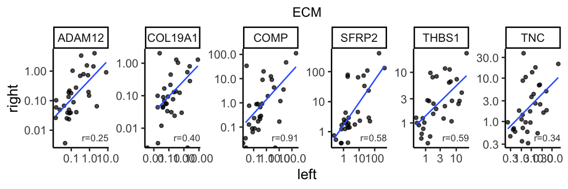 

ggsave(file.path(draft_fig_dir, "bilateral_cor_ECM_basket_genes.pdf"),
       width=7, height=1.7)  

inflam_corr <- gene_cor %>% dplyr::filter(basket == "Inflamm") %>%
  dplyr::mutate(formated=format(correlation, digit=2))

bilat_tpm %>% dplyr::filter(basket %in% c("Inflamm")) %>%
  ggplot(aes(x=L, y=R)) +
    geom_point(size=1, alpha=0.7) +
    geom_smooth(method="lm", linewidth=0.5, se=FALSE, alpha=0.5) +
    facet_wrap(~gene_name, scales="free", nrow=1) +
    geom_text(data=inflam_corr, aes(label=paste0("r=", formated)),
              x=Inf, y=-Inf, color="gray25", 
              hjust=1, vjust=-1, size=2.5) +
    theme_classic() +
    theme(plot.title=element_text(hjust=0.5, size=10)) +
    labs(x="left", y="right", title="Inflamm")  +
    scale_y_continuous(trans="log10") + 
    scale_x_continuous(trans="log10") 

ggsave(file.path(draft_fig_dir, "bilateral_cor_Inflamm_basket_genes.pdf"),
       width=7, height=1.7)  

complement_corr <- gene_cor %>% dplyr::filter(basket == "Complement") %>%
  dplyr::mutate(formated=format(correlation, digit=2))

bilat_tpm %>% dplyr::filter(basket %in% c("Complement")) %>%
  ggplot(aes(x=L, y=R)) +
    geom_point(size=1, alpha=0.7) +
    geom_smooth(method="lm", linewidth=0.5, se=FALSE, alpha=0.5) +
    facet_wrap(~gene_name, scales="free", nrow=1) +
    geom_text(data=complement_corr, aes(label=paste0("r=", formated)),
              x=Inf, y=-Inf, color="gray25", 
              hjust=1, vjust=-1, size=2.5) +
    theme_classic() +
    theme(plot.title=element_text(hjust=0.5, size=10)) +
    labs(x="left", y="right", title="Complement") +
    scale_y_continuous(trans="log10") + 
    scale_x_continuous(trans="log10")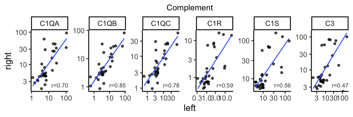 

ggsave(file.path(draft_fig_dir, "bilateral_cor_Complement_basket_genes.pdf"),
       width=7, height=1.7)  

ig_corr <- gene_cor %>% dplyr::filter(basket == "IG") %>%
  dplyr::mutate(formated=format(correlation, digit=2))

bilat_tpm %>% dplyr::filter(basket %in% c("IG")) %>%
  ggplot(aes(x=L, y=R)) +
    geom_point(size=1, alpha=0.7) +
    geom_smooth(method="lm", linewidth=0.5, se=FALSE, alpha=0.5) +
    facet_wrap(~gene_name, scales="free", nrow=1) +
    geom_text(data=ig_corr, aes(label=paste0("r=", formated)),
              x=Inf, y=-Inf, color="gray25", 
              hjust=1, vjust=-1, size=2.5) +
    theme_classic() +
    theme(plot.title=element_text(hjust=0.5, size=10)) +
    labs(x="left", y="right", title="IG") +
    scale_y_continuous(trans="log10") + 
    scale_x_continuous(trans="log10")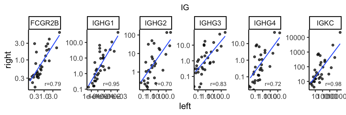 

ggsave(file.path(draft_fig_dir, "bilateral_cor_IG_basket_genes.pdf"),
       width=7, height=1.7)  

7.5.2 Per-basket by log sum

Here we calculate the per-basket bilateral correlation using basket scores (accumulated \(log_{10}(TPM+1)\)).

data <- comprehensive_df %>% 
  dplyr::select(Subject, location, `DUX4-M6-logSum`,
                `Inflamm-logSum`, `ECM-logSum`, `IG-logSum`,
                `Complement-logSum`) %>%
  gather(key=basket, value=scores, -Subject, -location) %>%
  spread(key=location, value=scores) %>%
  drop_na(L, R) %>%
  dplyr::mutate(basket=str_replace(basket, "-logSum", "")) %>%
  dplyr::mutate(basket=factor(basket, levels=c("DUX4-M6",
                                               "Inflamm", "ECM",
                                               "Complement", "IG")))

basket_cor <- data %>% group_by(basket) %>%
  summarise(cor=cor(L, R))

ggplot(data, aes(x=L, y=R)) +
  geom_point(size=1) +
  geom_smooth(method="lm", se=FALSE) +
    geom_abline(slope=1, intercept=0, color="grey50",
                linetype="dashed", alpha=0.5) +
    theme_classic() +
    facet_wrap(~basket, scale="free") +
    labs(title="Basket scroes bilateral correlation (Pearson)",
         x="Left", y="Right") +
    theme(plot.title = element_text(hjust = 0.5, size=10),
          axis.title = element_text(size=8)) +
    geom_text(data=basket_cor, aes(label=format(cor, digit=2)),
              x=Inf, y=-Inf, color="gray25", 
              hjust=1, vjust=-1)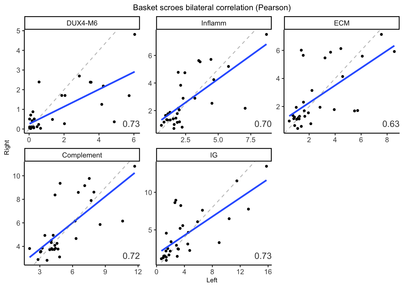

Figure 7.4: Basket score between the feft and Right TA muscles.

ggsave(file.path(draft_fig_dir, "bilateral_cor_baskets.pdf"),
       width=5, height=3.5)