8 Immune cell infiltrates signature
Please note that in the longitudinal study, we employed K-means clustering to identify five distinct clusters labeled as Mild, Moderate, IG-High, High, and Muscle-Low. Through this study, we have found that T cell proliferation, migration, and B cell-mediated immune responses are more prominent in severely affected muscles, specifically those labelled as “IG-high” and “High”. The objective of this chapter is as follows:
- Identify the enriched GO terms (biological processes) directly linked to T/B cells and circulating immunoglobulins in the longitudinal study (High or IG0high vs. control).
- Determine the differentially expressed genes (High vs. control) associated with the enriched GO terms (from step 1), and use heatmap visualization to observe the trend of an increase in gene expression across all longitudinal and bilateral samples, associated with the severity of FSHD (characterised by STIR status, fat fraction/infiltration percent) and/or complement scoring.
- Identify immune cell markers that are differentially expressed (High vs. control) using the IRIS database (Abbs 2009) as a source.
library(tidyverse)
library(DESeq2)
library(pheatmap)
library(kableExtra)
suppressPackageStartupMessages(library(writexl))
suppressPackageStartupMessages(library(knitr))
suppressPackageStartupMessages(library(kableExtra))
suppressPackageStartupMessages(library(purrr))
library(wesanderson)
library(latex2exp)

pkg_dir <- "/Users/cwon2/CompBio/Wellstone_BiLateral_Biopsy"
fig_dir <- file.path(pkg_dir, "figures", "immune-infiltration")
load(file.path(pkg_dir, "data", "bilat_dds.rda"))
load(file.path(pkg_dir, "data", "longitudinal_dds.rda"))
load(file.path(pkg_dir, "data", "bilat_MLpredict.rda"))
load(file.path(pkg_dir, "data", "comprehensive_df.rda"))
source(file.path(pkg_dir, "scripts", "viz_tools.R"))

# tidy annotation from two datasets
anno_gencode35 <- as.data.frame(rowData(bilat_dds)) %>%
  rownames_to_column(var="gencode35_id") %>% # BiLat study using Gencode 36
  dplyr::mutate(ens_id=str_replace(gencode35_id, "\\..*", "")) %>%
  dplyr::distinct(gene_name, .keep_all = TRUE)

anno_ens88 <- as.data.frame(rowData(longitudinal_dds)) %>%
  rownames_to_column(var="ens88_id") %>% # longitudinal study ens v88
  dplyr::mutate(ens_id=str_replace(gene_id, "\\..*", "")) %>%
  dplyr::distinct(gene_name, .keep_all = TRUE) %>%
  dplyr::select(ens88_id, ens_id, gene_name)
# insert class to bilat_dds
col_data <- colData(bilat_dds) %>% as.data.frame() %>%
  left_join(bilat_MLpredict, by="sample_id")
bilat_dds$class <- col_data$class

longitudinal_dds$STIR_status <- if_else(longitudinal_dds$STIR_rating > 0, "STIR+", "STIR-")

# color pal
col <- c("#ccece6", "#006d2c") # control vs. FSHD?
stir_pal <- c("STIR+" = "#006d2c", "STIR-" = "#ccece6")
complement_pal = c("3" = "#006d2c", "2" = "#66c2a4", "1" = "#ccece6")
8.1 Enriched biological processes directly associated with T/B cells
The code chunk below (1) obtains the enriched GO terms in more affected muscles from the longitudinal study, supplementary table 5, and (2) retains the enriched GO terms containing the terms including T cell, B cell, humoral, immunoglobulin, and complement. Total 20 terms are extracted.
high_enriched <- readxl::read_xlsx(file.path(pkg_dir, "extdata",
    "suppl_table_5_Candidate_Biomarkers_and_Enriched_Go.xlsx"),
    sheet=2, skip=2)

ig_enriched <- readxl::read_xlsx(file.path(pkg_dir, "extdata",
    "suppl_table_5_Candidate_Biomarkers_and_Enriched_Go.xlsx"),
    sheet=4, skip=2)

moderate_enriched <- readxl::read_xlsx(file.path(pkg_dir, "extdata",
    "suppl_table_5_Candidate_Biomarkers_and_Enriched_Go.xlsx"),
    sheet=6, skip=2)

# get the lymphocyte related GO ID
infiltrates_go <- high_enriched %>%
  dplyr::filter(str_detect(term, "T cell|B cell|humoral|immunoglobulin|complement"))

infiltrates_go %>%
  dplyr::select(category, over_represented_pvalue, term) %>%
  dplyr::rename(pvalue = over_represented_pvalue) %>%
  dplyr::mutate(pvalue = format(pvalue, scientific = TRUE)) %>%
  dplyr::arrange(category) %>%
  kbl(caption="Enriched biological process GO terms (n=20)  related to T/B cells, humoral immune response, and immunoglobulin domains. Identified using the longitudinal IG-High and High samples (vs. controls).") %>%
kable_paper("hover", full_width = F)| category | pvalue | term |
|---|---|---|
| GO:0002455 | 4.391414e-10 | humoral immune response mediated by circulating immunoglobulin |
| GO:0002460 | 6.665762e-09 | adaptive immune response based on somatic recombination of immune receptors built from immunoglobulin superfamily domains |
| GO:0002920 | 2.865839e-11 | regulation of humoral immune response |
| GO:0006956 | 4.086619e-10 | complement activation |
| GO:0006957 | 1.965806e-04 | complement activation, alternative pathway |
| GO:0006958 | 1.619492e-10 | complement activation, classical pathway |
| GO:0006959 | 1.158839e-15 | humoral immune response |
| GO:0010818 | 2.450256e-09 | T cell chemotaxis |
| GO:0016064 | 1.175922e-08 | immunoglobulin mediated immune response |
| GO:0019724 | 1.380039e-08 | B cell mediated immunity |
| GO:0030449 | 7.071256e-11 | regulation of complement activation |
| GO:0031295 | 1.531739e-04 | T cell costimulation |
| GO:0042098 | 5.735434e-06 | T cell proliferation |
| GO:0042102 | 4.877625e-05 | positive regulation of T cell proliferation |
| GO:0042110 | 6.083250e-07 | T cell activation |
| GO:0042129 | 1.273162e-05 | regulation of T cell proliferation |
| GO:0050863 | 3.541698e-08 | regulation of T cell activation |
| GO:0050870 | 1.090819e-06 | positive regulation of T cell activation |
| GO:0072678 | 1.727781e-11 | T cell migration |
| GO:2000404 | 1.335915e-05 | regulation of T cell migration |
Display the p-values yielded by GSEA:
df <- infiltrates_go %>%
  dplyr::select(category, term, over_represented_pvalue) %>%
  arrange(term) %>%
  left_join(dplyr::select(ig_enriched, category, over_represented_pvalue),
            by="category", suffix=c(".High", ".IG-High")) %>%
  tidyr::gather(key=class, value=pvalue, -category, -term) %>%
  dplyr::mutate(class = str_replace(class,
                                    "over_represented_pvalue.", ""),
                term = str_trunc(term, 45),
                class = factor(class, levels=c("IG-High", "High"))) %>%
  dplyr::mutate(log10pvalue = -log10(pvalue))

cat_levels <- df %>% dplyr::filter(class == "High") %>%
  dplyr::arrange(category) %>% pull(term)

df %>% dplyr::mutate(term=factor(term, levels=cat_levels)) %>%
  #dplyr::mutate(term = factor(term,levels=cat_levels)) %>%
  ggplot(aes(x=class, y=term)) +
    geom_point(aes(size=log10pvalue), color="red1", alpha=0.7,
               show.legend = FALSE) +
    theme_minimal() +
  labs(title="Enriched GO terms related to T/B cells and immunoglobulins") +
  theme(axis.title.x = element_blank(),
        plot.title = element_text(hjust=1, size=9.5),
        axis.title.y = element_blank())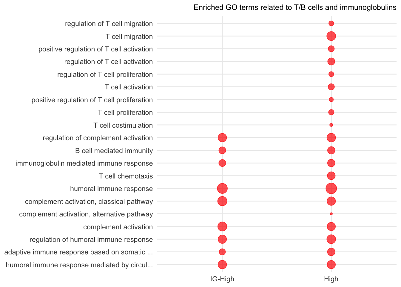
Figure 8.1: Enriched GO terms related to T and B cells and immunoglobulin domains. Red dots present the p-value of enriched GO terms in IG or High samples.
8.2 Significant genes associated with the T/B-associated enriched GO terms
The code chunk below identifies significantly expressed genes in High or IG-High (compared to the controls) that are associated with the enriched GO terms obtained previously.
Results: Total 95 B/T cell immunity response significant markers are identified.
high_sig <- readxl::read_xlsx(file.path(pkg_dir, "extdata",
    "suppl_table_5_Candidate_Biomarkers_and_Enriched_Go.xlsx"),
    sheet=1, skip=3) %>%
  dplyr::select(gene_name, gencode_id) %>%
  dplyr::mutate(ens_id = str_replace(gencode_id, "\\..*", ""))

ig_sig <- readxl::read_xlsx(file.path(pkg_dir, "extdata",
    "suppl_table_5_Candidate_Biomarkers_and_Enriched_Go.xlsx"),
    sheet=3, skip=3) %>%
  dplyr::select(gene_name, gencode_id) %>%
  dplyr::mutate(ens_id = str_replace(gencode_id, "\\..*", ""))
sig <- bind_rows(high_sig, ig_sig) %>%
  dplyr::distinct(gene_name, .keep_all=TRUE)

## keep the genes that involved in the infiltrates_go
gene2cat <- goseq::getgo(sig$ens_id, "hg38", "ensGene", fetch.cats = "GO:BP")
names(gene2cat) <- sig$ens_id
cat2gene <- goseq:::reversemapping(gene2cat)[infiltrates_go$category]
infiltrates_act <- map_dfr(cat2gene, function(cat_gene) {
  sig %>% dplyr::filter(ens_id %in% cat_gene)
}, .id="category") %>%
  arrange(category) %>%
  left_join(dplyr::select(infiltrates_go, category, term), by="category") %>%
  dplyr::rename(GOID = category) %>%
  distinct(gene_name, .keep_all=TRUE) %>%
  dplyr::rename(gene_id = gencode_id) %>%
  #arrange(gene_name) %>%
  dplyr::mutate(category = case_when(
    str_detect(term, "T cell") ~ "T cell migration / activation",
    str_detect(term, "humoral|complement") ~ "B cell mediated / humoral immune response",
    str_detect(term, "adaptive") ~ "adaptive immune response (IG domains)"
  )) %>%
  arrange(category, gene_name)
8.2.1 Heatmap: Longitudinal study
We have employed a heatmap to visualize the trend of increased expression levels for the 95 immune signature genes previously identified to be associated with enriched T/B and IG Gene Ontology (GO) terms. The order of the samples in the heatmap is arranged as Control, Mild, Moderate, IG-High, High, and Muscle-low.
cluster_color <- c(Control="#ff7f00",
                    Mild="#a65628",
                    Moderate="#f781bf",
                    `IG-High`="#984ea3", High="#e41a1c",
                   `Muscle-Low`="#377eb8")
category_color <- wes_palette("Darjeeling2", n=4)[c(1,3,4)]
names(category_color) <- levels(factor(infiltrates_act$category))
col <- c("#ccece6", "#006d2c")
stir_pal <- c("STIR+" = "#006d2c", "STIR-" = "#ccece6")
complement_pal = c("3" = "#006d2c", "2" = "#66c2a4", "1" = "#ccece6")
# column annotation: class, fat fraction, STIR rating, and histophatology

annotation_col <- colData(longitudinal_dds) %>% as.data.frame() %>%
  dplyr::select(cluster, fat_fraction, STIR_status,
                #STIR_rating,
                Pathology.Score) %>%
  dplyr::rename(class=cluster, `STIR+/-` = STIR_status,
                `fat fraction`=fat_fraction,
                `histopathology` = Pathology.Score) %>%
  dplyr::mutate(`STIR+/-` = factor(`STIR+/-`))
# column annotation color
ann_cor <-  list(class = cluster_color, category = category_color,
                 `STIR+/-` = stir_pal,
                 `fat fraction` = col,
                 `histopathology` = col)
markers_heatmp_group_by_types_class(markers = infiltrates_act,
                                    dds = longitudinal_dds,
                                    factor = "cluster",
                                    annotation_col = annotation_col,
                                    ann_cor = ann_cor,
                                    annotation_legend=TRUE)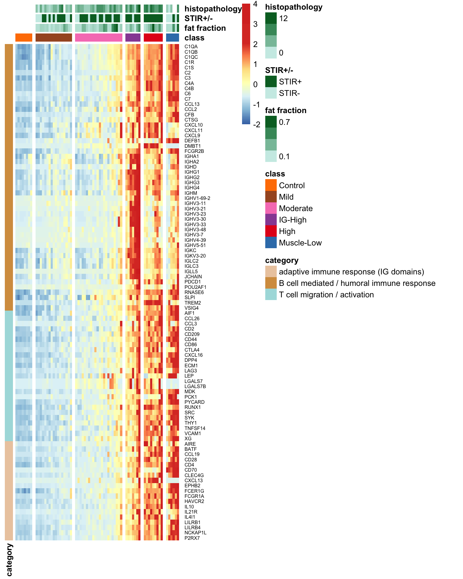
Figure 8.2: Heatmap demonstrating the increased expression trend for 95 previously identifed T/B and IG domain related genes on more affected muscle. Color presented the row-wised z-score of expression levels.
8.2.2 Heatmap: bilateral study
The code chunk below generates a heatmap depicting the expression levels of the 95 immune signature genes from the bilateral samples. Noted that the samples are ordered based on their classification into Control-like and Moderate+, determined by ML-based classification, and Muscle-Low based on the low expression levels of muscle markers.
annotation_col <- comprehensive_df %>%
  drop_na(class) %>%
  dplyr::select(sample_id, class, Fat_Infilt_Percent, STIR_status,
                `Cumulative Score`, `Complement Scoring`) %>%
  dplyr::rename(`fat percent` = Fat_Infilt_Percent,
                `STIR+/-` = STIR_status,
                `histopathology` = `Cumulative Score`) %>%
  column_to_rownames(var="sample_id") %>%
  dplyr::mutate(`Complement Scoring` = factor(`Complement Scoring`,
                                              levels=c("3", "2", "1")))

class_color <- c(`Control-like`="#a65628",
                 `Moderate+`="#984ea3",
                 `Muscle-Low`="#377eb8")
ann_cor <- list(class = class_color, category = category_color,
                `fat percent` = col,
                `STIR+/-` = stir_pal,
                `histopathology` = col,
                `Complement Scoring` = complement_pal)

markers <- infiltrates_act %>%
  left_join(dplyr::select(anno_gencode35, ens_id, gencode35_id),
            by="ens_id") %>%
  dplyr::select(-gene_id) %>%
  dplyr::rename(gene_id = gencode35_id) %>%
  drop_na(gene_id)

markers_heatmp_group_by_types_class(markers = markers,
                                    dds = bilat_dds,
                                    factor = "class",
                                    annotation_legend=TRUE,
                                    annotation_col = annotation_col,
                                    border_color = "transparent",
                                    ann_cor = ann_cor)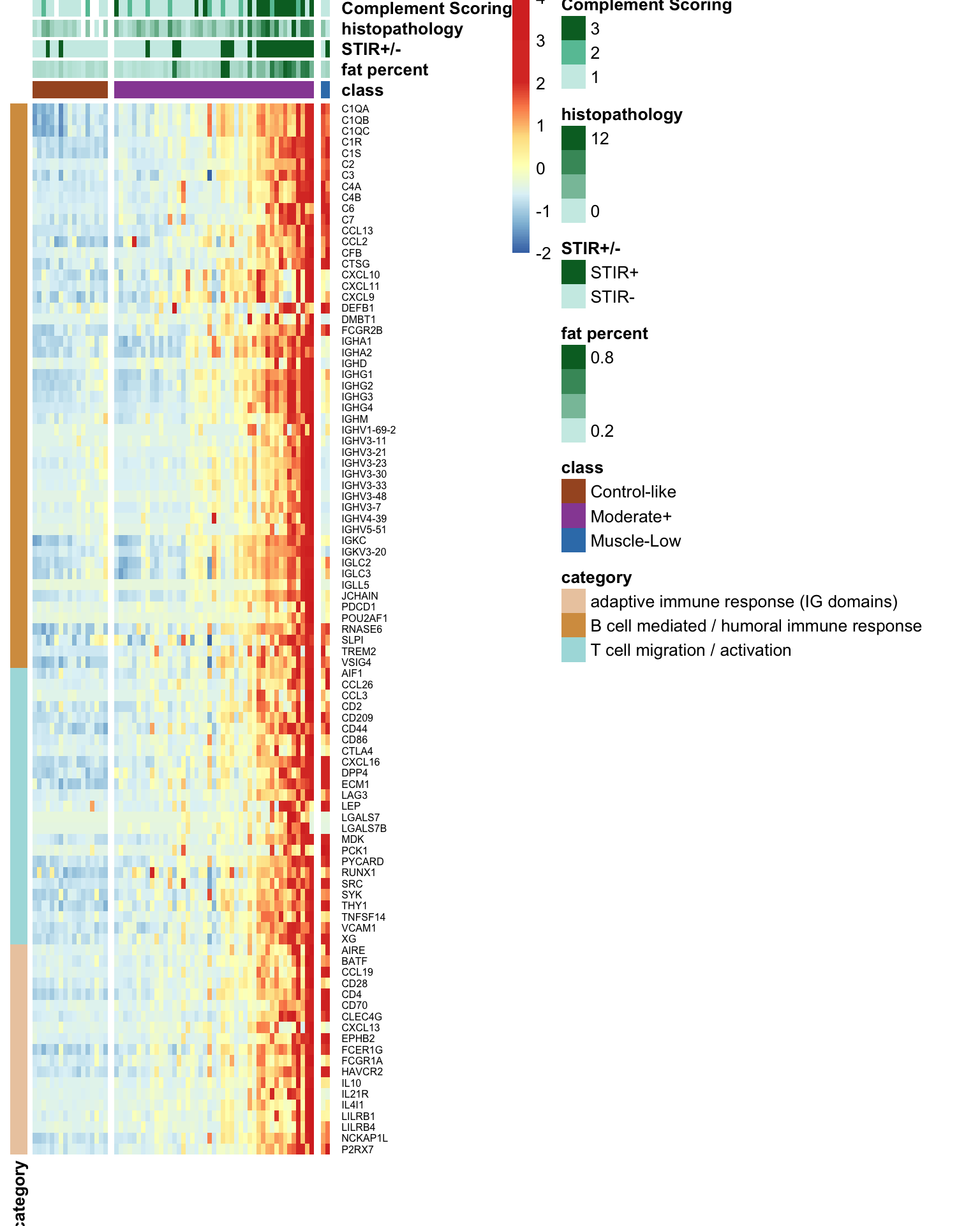
8.3 Immune cell infiltrate signature
Using a generic cell-type marker dataset from the immune response in silico (IRIS) (Abbas 2009) and longitudinal cohort, we detected 63 immune cell markers whose expression levels are significantly elevated in more affected muscles. With additional significant immunity-related markers, including such as cytokine receptors in B cells (IL-4R, IL-21R), STAT6, Leukocyte immunoglobulin-like receptor B family (LILRB4, LILRB5), T cell surface antigens (CD2 and CD4), T and B cell interaction and migration (CCL19), and STAT6, we demonstrated a immune cell infiltrate signatures in both longitudinal and bilateral samples.
Code chunk below identified 63 immune cell markers as a subset of the IRIS database (Abbas 2009).
library(PLIER)
data(bloodCellMarkersIRISDMAP)
# about 860 markers
blood_iris <- as.data.frame(bloodCellMarkersIRISDMAP) %>%
  rownames_to_column(var="gene_name") %>%
  dplyr::select(gene_name, starts_with("IRIS")) %>%
  dplyr::filter(rowSums(across(where(is.numeric))) > 0)

# 63 are DE in High, longitudinal cohort
sig_blood_iris <- high_sig %>%
  inner_join(blood_iris, by="gene_name")
category <- names(sig_blood_iris)[4:ncol(sig_blood_iris)]
sig_blood_iris$category <-
  apply(sig_blood_iris[, 4:ncol(sig_blood_iris)], 1,
        function(x) {
    tmp <- if_else(unlist(as.vector(x)) == 1, TRUE, FALSE)
    return(category[tmp][1])
       })

sig_blood_iris  <- sig_blood_iris %>%
  dplyr::select(gene_name, gencode_id, ens_id, category) %>%
  dplyr::rename(gene_id = gencode_id) %>%
  dplyr::mutate(category = str_replace(category, "IRIS_", "")) %>%
  dplyr::mutate(category = str_replace(category, "\\-.*", "")) %>%
  arrange(category, gene_name) %>%
  dplyr::mutate(category = factor(category,
                                  levels = c("Bcell", "CD4Tcell", "CD8Tcell",
                                             "DendriticCell",
                                             "Monocyte", "Neutrophil",
                                             "NKcell", "PlasmaCell")))

# modification: do not consider those "other" markers
# add others: IL-4R, IL-21R, LILRB4, LILRB5, CD2, CD4, CCL19
#others <- data.frame(gene_name = c("IL4R", "IL21R", "LILRB4",
#                                   "LILRB5",
#                                   "CD2", "CD4", "CCL19", "STAT6")) %>%
#  left_join(anno_ens88, by="gene_name") %>%
#  dplyr::rename(gene_id = ens88_id) %>%
#  add_column(category="Others") %>%
#  arrange(gene_name)
8.3.1 Heamap: the longitudinal study
The following heatmap illustrates that there is a tendency of higher expression levels in muscles that are more affected.
cluster_color <- c(Control="#ff7f00",
                    Mild="#a65628",
                    Moderate="#f781bf",
                    `IG-High`="#984ea3", High="#e41a1c",
                   `Muscle-Low`="#377eb8")


annotation_col <- colData(longitudinal_dds) %>% as.data.frame() %>%
  dplyr::select(cluster, fat_fraction, STIR_status,
                Pathology.Score) %>%
  dplyr::rename(class=cluster,
                `fat fraction`=fat_fraction,
                `STIR+/-` = STIR_status,
                `histopathology` = Pathology.Score) %>%
  dplyr::mutate(`STIR+/-` = factor(`STIR+/-`))

category_color <- wes_palette("Darjeeling1", n=8, typ="continuous")[1:8]
names(category_color) <- levels(sig_blood_iris$category)

ann_cor <-  list(class = cluster_color,
                 category = category_color,
                 `fat fraction` = col,
                 `STIR+/-` = stir_pal,
                 `histopathology` = col)
# heatmap
markers_heatmp_group_by_types_class(markers = sig_blood_iris,
                                    dds = longitudinal_dds,
                                    factor = "cluster",
                                    border_color = "transparent",
                                    annotation_col = annotation_col,
                                    ann_cor = ann_cor)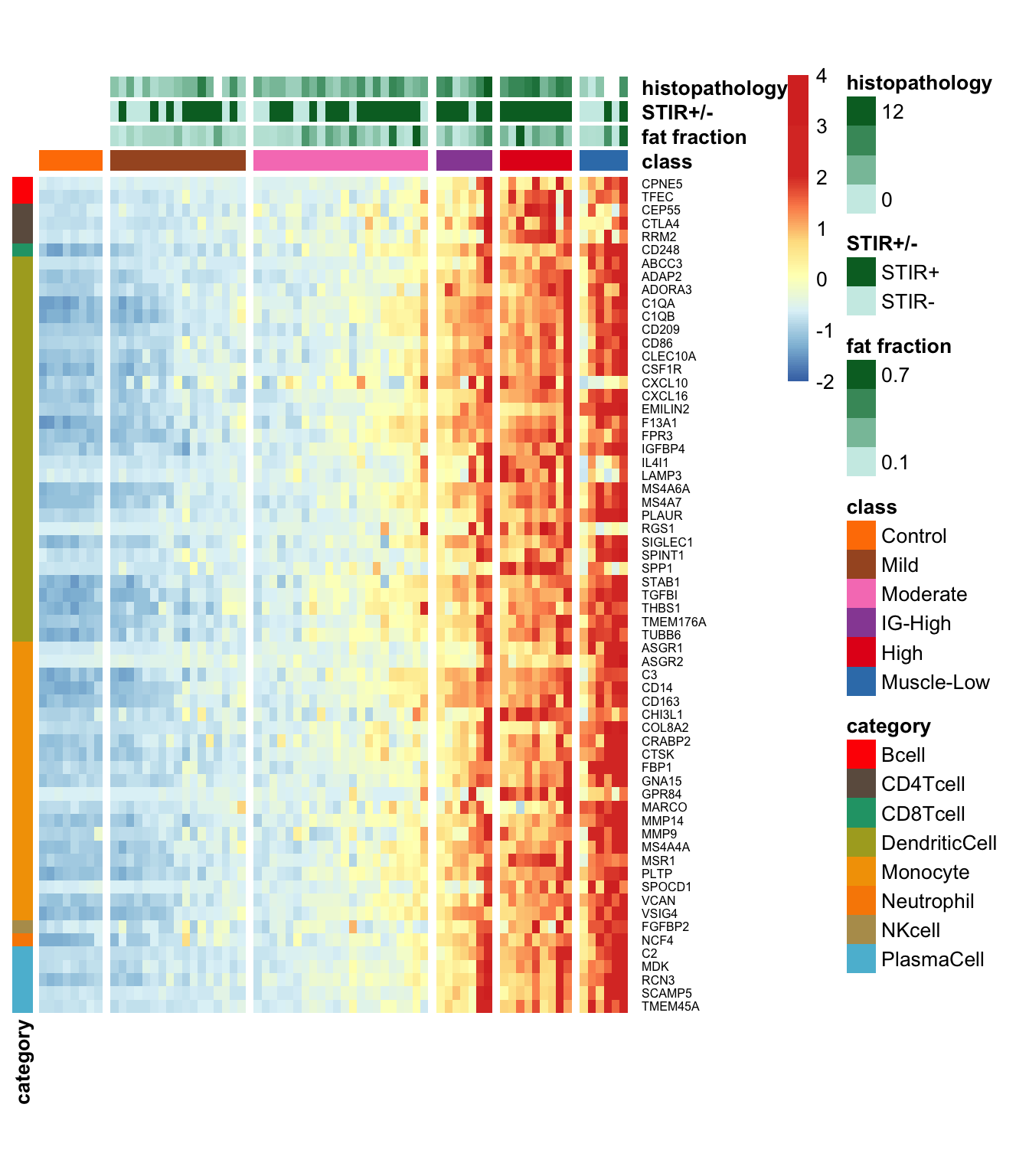
Figure 8.3: Heapmap demonstrating the expression levels (by row-wise z-score of log10(TPM++1) in the longitudinal study.
8.3.2 Heatmap: Bilateral study
The heatmap for the bilateral study below incorporates the complement scoring.
annotation_col <- comprehensive_df %>%
  drop_na(class) %>%
  dplyr::select(sample_id, class, Fat_Infilt_Percent, STIR_status,
                `Cumulative Score`, `Complement Scoring`) %>%
  dplyr::rename(`fat percent` = Fat_Infilt_Percent,
                `STIR+/-` = STIR_status,
                `histopathology` = `Cumulative Score`) %>%
  column_to_rownames(var="sample_id") %>%
  dplyr::mutate(`Complement Scoring` = factor(`Complement Scoring`))

class_color <- c(`Control-like`="#a65628",
                    `Moderate+`="#984ea3",
                    `Muscle-Low`="#377eb8")
ann_cor <- list(class = class_color, category = category_color,
                `fat percent` = col,
                `STIR+/-` = stir_pal,
                `histopathology` = col,
                `Complement Scoring` = complement_pal)

# update sig_blood_iris gene_id to gencode35_id
tmp <- sig_blood_iris %>%
  left_join(dplyr::select(anno_gencode35, ens_id, gencode35_id),
            by="ens_id") %>%
  dplyr::select(-gene_id) %>%
  dplyr::rename(gene_id = gencode35_id)

markers_heatmp_group_by_types_class(markers = tmp,
                                    dds = bilat_dds,
                                    factor = "class",
                                    border_color = "transparent",
                                    annotation_col = annotation_col,
                                    ann_cor = ann_cor )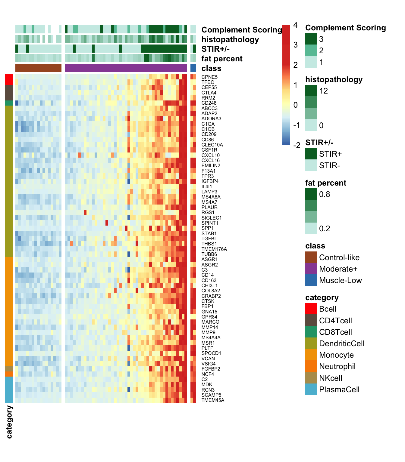
8.3.3 DE immune marker in the Bilat corhort
We compared the Control-like and Moderate+ samples in the Bilat cohort to determine which the immune cell-type genes in the IRIS dataset are differentially expressed.
sub_dds <- bilat_dds[, bilat_dds$class %in% c("Control-like", "Moderate+")]
sub_dds$class <- factor(sub_dds$class)
design(sub_dds) <- ~ class
sub_dds <- DESeq(sub_dds)
immune_signature_gene <- sig_blood_iris %>%
  left_join(dplyr::select(anno_gencode35, ens_id, gencode35_id),
            by="ens_id") %>%
  dplyr::select(-gene_id) %>%
  dplyr::rename(gene_id = gencode35_id)

res <- results(sub_dds, lfcThreshold = 0.5) %>%
  as.data.frame() %>%
  rownames_to_column(var="gene_id") %>%
  dplyr::filter(padj < 0.05, log2FoldChange > 0) %>%
  inner_join(immune_signature_gene, by="gene_id")

res %>%
  dplyr::select(gene_id, gene_name, log2FoldChange, category) %>%
  kbl(caption='44 IRIS immune markers that are significently expressed in Modereate+ samples relative to the control-like samples.') %>%
kable_styling()| gene_id | gene_name | log2FoldChange | category |
|---|---|---|---|
| ENSG00000002933.9 | TMEM176A | 1.545149 | DendriticCell |
| ENSG00000038427.16 | VCAN | 1.254348 | Monocyte |
| ENSG00000038945.15 | MSR1 | 1.631995 | Monocyte |
| ENSG00000060558.4 | GNA15 | 1.732585 | Monocyte |
| ENSG00000078081.8 | LAMP3 | 3.208762 | DendriticCell |
| ENSG00000090104.12 | RGS1 | 3.254608 | DendriticCell |
| ENSG00000090659.18 | CD209 | 1.687079 | DendriticCell |
| ENSG00000100979.15 | PLTP | 1.539781 | Monocyte |
| ENSG00000100985.7 | MMP9 | 2.886832 | Monocyte |
| ENSG00000104951.16 | IL4I1 | 3.070091 | DendriticCell |
| ENSG00000105967.16 | TFEC | 1.733737 | Bcell |
| ENSG00000108846.16 | ABCC3 | 2.173910 | DendriticCell |
| ENSG00000110077.14 | MS4A6A | 1.591415 | DendriticCell |
| ENSG00000110079.18 | MS4A4A | 1.647453 | Monocyte |
| ENSG00000114013.16 | CD86 | 1.609474 | DendriticCell |
| ENSG00000118785.14 | SPP1 | 4.957166 | DendriticCell |
| ENSG00000124491.16 | F13A1 | 1.777443 | DendriticCell |
| ENSG00000124772.12 | CPNE5 | 2.192108 | Bcell |
| ENSG00000125730.17 | C3 | 1.689339 | Monocyte |
| ENSG00000132205.11 | EMILIN2 | 1.440005 | DendriticCell |
| ENSG00000132514.13 | CLEC10A | 1.486597 | DendriticCell |
| ENSG00000133048.13 | CHI3L1 | 2.736904 | Monocyte |
| ENSG00000137441.8 | FGFBP2 | 2.177403 | NKcell |
| ENSG00000137801.11 | THBS1 | 1.995249 | DendriticCell |
| ENSG00000139572.4 | GPR84 | 2.554428 | Monocyte |
| ENSG00000143320.9 | CRABP2 | 1.922802 | Monocyte |
| ENSG00000143387.13 | CTSK | 1.456861 | Monocyte |
| ENSG00000155659.15 | VSIG4 | 1.435979 | Monocyte |
| ENSG00000157227.13 | MMP14 | 1.302515 | Monocyte |
| ENSG00000161921.16 | CXCL16 | 1.362402 | DendriticCell |
| ENSG00000163599.17 | CTLA4 | 2.343052 | CD4Tcell |
| ENSG00000166278.15 | C2 | 2.486130 | PlasmaCell |
| ENSG00000166927.13 | MS4A7 | 1.716174 | DendriticCell |
| ENSG00000169245.6 | CXCL10 | 2.637787 | DendriticCell |
| ENSG00000170458.14 | CD14 | 1.377451 | Monocyte |
| ENSG00000171812.13 | COL8A2 | 1.870228 | Monocyte |
| ENSG00000171848.15 | RRM2 | 2.263203 | CD4Tcell |
| ENSG00000173369.17 | C1QB | 1.939756 | DendriticCell |
| ENSG00000173372.17 | C1QA | 1.684487 | DendriticCell |
| ENSG00000177575.12 | CD163 | 1.736284 | Monocyte |
| ENSG00000181458.10 | TMEM45A | 1.878089 | PlasmaCell |
| ENSG00000182578.14 | CSF1R | 1.345719 | DendriticCell |
| ENSG00000187474.5 | FPR3 | 1.862982 | DendriticCell |
| ENSG00000198794.12 | SCAMP5 | 1.762450 | PlasmaCell |
8.4 Complement scoring vs. immune cell infiltrates signature
The earlier mentioned 63 immune cell markers contribute to characterizing the signature of immune cell infiltration. The following code calculates the Spearman correlation coefficient between complement scoring and immune cell signature (average \(\log_{10}\)TPM of 63 immune cell markers), which yields a value of 0.456.
tpm <- assays(bilat_dds[immune_signature_gene$gene_id])[["TPM"]]

signature <- colMeans(log10(tpm+1)) %>% as.data.frame() %>%
  rownames_to_column(var="sample_id")
names(signature)[2] <- "avg_tpm"

tmp_df <- comprehensive_df %>%
  dplyr::select(sample_id, `Complement Scoring`, `STIR_status`,
                `STIR_RATING`) %>%
  left_join(signature, by="sample_id") %>%
  drop_na(`Complement Scoring`, `avg_tpm`)

# Spearman correlation between complement and immune infiltrate signatures
tmp_df %>%
  drop_na(`Complement Scoring`, `avg_tpm`) %>%
  dplyr::select(`Complement Scoring`, `avg_tpm`) %>%
  corrr::correlate(., method="spearman")
#> # A tibble: 2 × 3
#>   term               `Complement Scoring` avg_tpm
#>   <chr>                             <dbl>   <dbl>
#> 1 Complement Scoring               NA       0.454
#> 2 avg_tpm                           0.454  NA
tmp_df %>%
  drop_na(`Complement Scoring`, `avg_tpm`) %>%
  dplyr::mutate(`Complement Scoring`= factor(`Complement Scoring`)) %>%
  ggplot(aes(x=`Complement Scoring`, y=avg_tpm)) +
    geom_boxplot(width=0.5, outlier.shape = NA) +
    geom_dotplot(aes(fill=`Complement Scoring`),
                 binaxis='y', stackdir='center',
                 show.legend = FALSE, alpha=0.8,
                 stackratio=1.5, dotsize=1.5) +
    theme_minimal()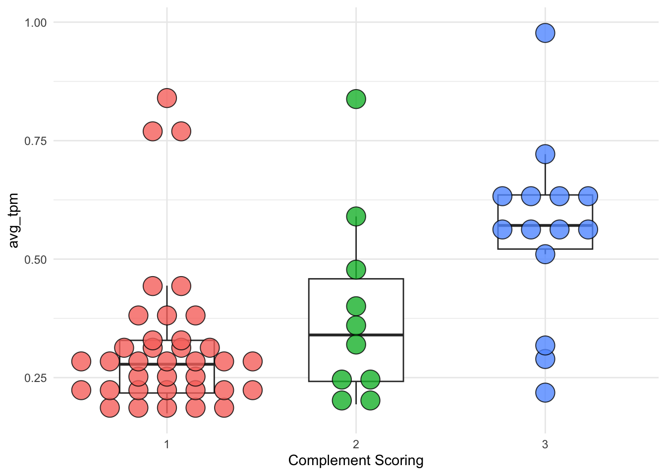
Figure 8.4: Dotplot of immune cell infiltrates signature (presented by average TPM) groups by complement scoring 1, 2, and 3.
8.5 STIR status vs. immune cell infiltrates signature
The elevated immune cell signatures is associated with with STIR status: Wilcox test p-value = \(2.9e-6\).
tmp_df %>%
  drop_na(`STIR_status`, `avg_tpm`) %>%
  ggplot(aes(x=`STIR_status`, y=avg_tpm)) +
    geom_boxplot(width=0.5, outlier.shape = NA) +
    geom_dotplot(aes(fill=`STIR_status`),
                 binaxis='y', stackdir='center',
                 show.legend = FALSE,
                 stackratio=1.5, dotsize=1.5, alpha=0.7) +
    theme_minimal()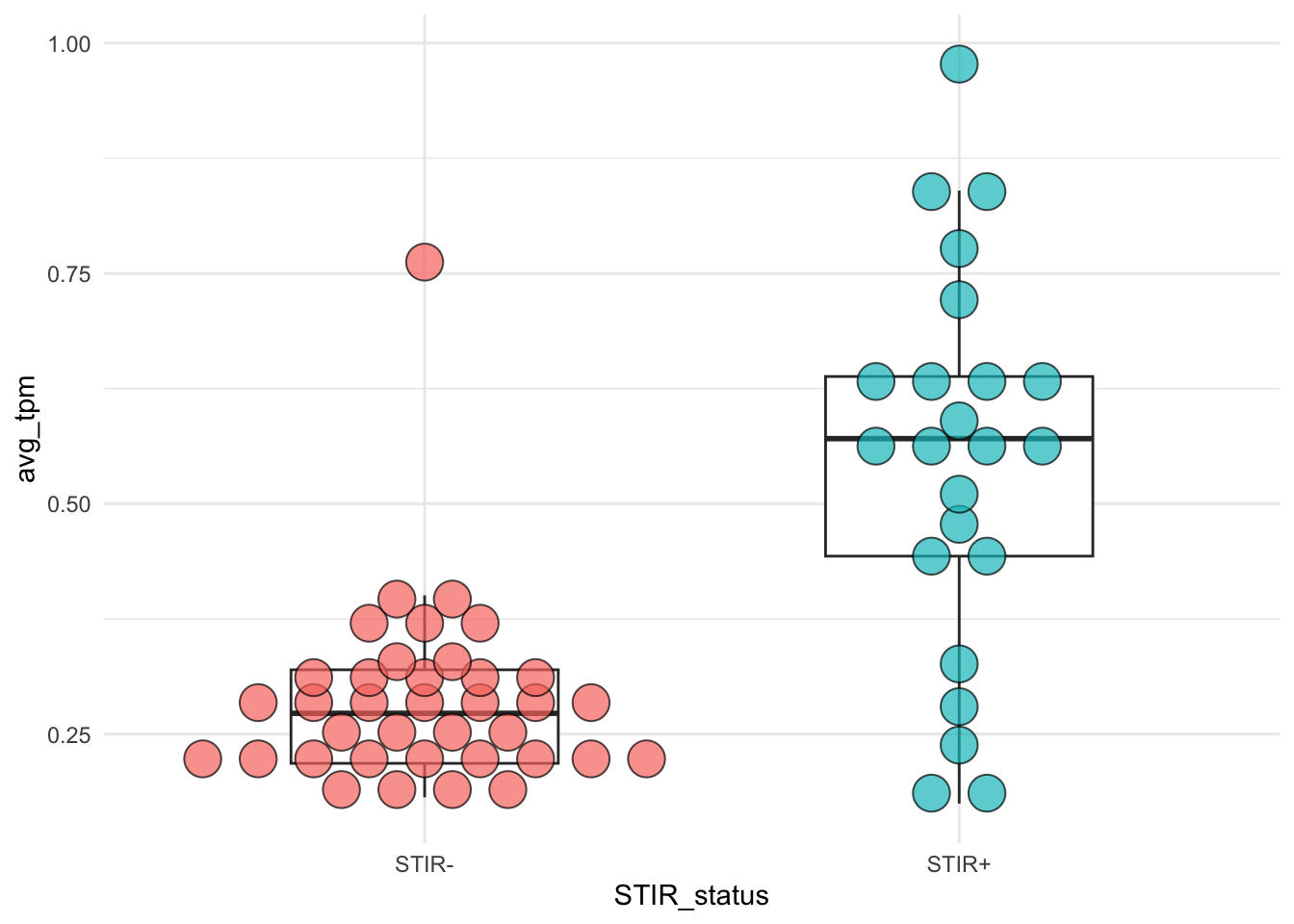
# wilcox.test
x <- tmp_df %>%
  drop_na(`STIR_status`, `avg_tpm`) %>%
  dplyr::select(sample_id, `STIR_status`, `avg_tpm`) %>%
  spread(key=STIR_status, value=avg_tpm)
wilcox.test(x$`STIR-`, x$`STIR+` )
#>
#>  Wilcoxon rank sum exact test
#>
#> data:  x$`STIR-` and x$`STIR+`
#> W = 134, p-value = 2.902e-06
#> alternative hypothesis: true location shift is not equal to 0
8.6 Bilateral comparison analysis for the immune cell infiltrate markers
8.6.1 63 significant immune cell markers
In the preceding section, we uncovered a distinctive signature of immune cell infiltrates defined by 63 immune cell markers within the longitudinal study. Now, calculate the expression correlation of these markers between the left and right muscles in the bilateral study.
The code below displays the tools to compute the correlation between L and R muscles on the immune cell infiltrate markers.
col_data <- colData(bilat_dds) %>% as.data.frame()
# convert gene_id to Gencode35
markers <- sig_blood_iris %>%
  left_join(dplyr::select(anno_gencode35, ens_id, gencode35_id),
            by="ens_id") %>%
  dplyr::select(-gene_id) %>%
  dplyr::rename(gene_id = gencode35_id)

.markers_bilateral_correlation <- function(markers, dds) {
  tpm <- assays(dds[markers$gene_id])[["TPM"]] %>% t(.) %>%
      as.data.frame() %>%
      rownames_to_column(var="sample_id") %>%
      gather(key=gene_id, value=TPM, -sample_id) %>%
      left_join(dplyr::select(col_data, sample_id, location,
                              Subject), by="sample_id") %>%
      dplyr::select(-sample_id) %>%
      spread(key=location, value=TPM) %>%
      drop_na(L, R)
  gene_cor <- tpm %>%
    dplyr::mutate(L_log = log10(L+1), R_log=log10(R+1)) %>%
    group_by(gene_id) %>%
    summarise(Pearson_by_TPM=cor(L, R),
              Pearson_by_log10TPM = cor(L_log, R_log)) %>%
    dplyr::left_join(markers, by="gene_id") %>%
    arrange(desc(Pearson_by_log10TPM)) %>%
    dplyr::relocate(gene_name, .after=gene_id)

  return(gene_cor)
}

.avg_TPM_by_class <- function(markers, dds) {
   avg_TPM <- map_dfc(levels(dds$class), function(x) {
     assays(dds[markers$gene_id])[["TPM"]][, dds$class == x] %>%
       rowMeans(.)
   }) %>%
     tibble::add_column(gene_id = markers$gene_id) %>%
     dplyr::rename_with(~paste0(levels(dds$class), " avg TPM"),
                        starts_with("..."))
}
Display the correlation and average TPM grouped by ML-based classes.
gene_cor_63 <- .markers_bilateral_correlation(markers=markers,
                                           dds=bilat_dds) %>%
  dplyr::left_join(.avg_TPM_by_class(markers = markers, dds=bilat_dds),
                   by="gene_id") %>%
  arrange(category)

gene_cor_63 %>%
  dplyr::select(-Pearson_by_TPM) %>%
  kbl(caption="Sixty-three significant immune cell markers correlation analysis between left and right biopsied muscles. The Peason correlation coefficients are compuated using the expression levels presented by Log10(TPM+1).") %>%
kable_styling()| gene_id | gene_name | Pearson_by_log10TPM | ens_id | category | Control-like avg TPM | Moderate+ avg TPM | Muscle-Low avg TPM |
|---|---|---|---|---|---|---|---|
| ENSG00000124772.12 | CPNE5 | 0.8373333 | ENSG00000124772 | Bcell | 0.0443273 | 0.3835624 | 1.0004216 |
| ENSG00000105967.16 | TFEC | 0.8176975 | ENSG00000105967 | Bcell | 0.0234566 | 0.1235314 | 0.1023323 |
| ENSG00000138180.16 | CEP55 | 0.7993619 | ENSG00000138180 | CD4Tcell | 0.0348918 | 0.1666287 | 0.2252888 |
| ENSG00000163599.17 | CTLA4 | 0.7880751 | ENSG00000163599 | CD4Tcell | 0.0315704 | 0.2644233 | 0.1854032 |
| ENSG00000171848.15 | RRM2 | 0.6609791 | ENSG00000171848 | CD4Tcell | 0.0090876 | 0.0662736 | 0.1102069 |
| ENSG00000174807.4 | CD248 | 0.6261514 | ENSG00000174807 | CD8Tcell | 14.3514643 | 48.2904687 | 253.0578657 |
| ENSG00000114013.16 | CD86 | 0.8269231 | ENSG00000114013 | DendriticCell | 0.0663682 | 0.3421849 | 0.4462872 |
| ENSG00000132514.13 | CLEC10A | 0.8181479 | ENSG00000132514 | DendriticCell | 0.3866177 | 1.7920233 | 3.3907985 |
| ENSG00000173369.17 | C1QB | 0.8099608 | ENSG00000173369 | DendriticCell | 2.0357169 | 13.7189810 | 28.4657562 |
| ENSG00000110077.14 | MS4A6A | 0.8063214 | ENSG00000110077 | DendriticCell | 0.4436241 | 2.1606915 | 3.6416739 |
| ENSG00000166927.13 | MS4A7 | 0.7842506 | ENSG00000166927 | DendriticCell | 0.2090296 | 1.1084212 | 1.9491638 |
| ENSG00000124491.16 | F13A1 | 0.7788406 | ENSG00000124491 | DendriticCell | 2.0078292 | 12.2302448 | 21.8912499 |
| ENSG00000182578.14 | CSF1R | 0.7750512 | ENSG00000182578 | DendriticCell | 0.7874655 | 3.3187330 | 7.1733571 |
| ENSG00000282608.2 | ADORA3 | 0.7736084 | ENSG00000282608 | DendriticCell | 0.0386997 | 0.1584448 | 0.2628639 |
| ENSG00000173372.17 | C1QA | 0.7445602 | ENSG00000173372 | DendriticCell | 3.4317578 | 19.1178534 | 52.6300218 |
| ENSG00000161921.16 | CXCL16 | 0.7398670 | ENSG00000161921 | DendriticCell | 0.3268772 | 1.4080810 | 5.0737114 |
| ENSG00000010327.10 | STAB1 | 0.7266172 | ENSG00000010327 | DendriticCell | 1.5300961 | 5.3923377 | 17.3660509 |
| ENSG00000078081.8 | LAMP3 | 0.7185273 | ENSG00000078081 | DendriticCell | 0.0108336 | 0.1663221 | 0.2174447 |
| ENSG00000090104.12 | RGS1 | 0.7173044 | ENSG00000090104 | DendriticCell | 0.0130089 | 0.2018628 | 0.1915478 |
| ENSG00000184060.11 | ADAP2 | 0.7103740 | ENSG00000184060 | DendriticCell | 0.3838474 | 1.1441190 | 3.2110364 |
| ENSG00000104951.16 | IL4I1 | 0.6975342 | ENSG00000104951 | DendriticCell | 0.0220052 | 0.3013386 | 0.1689496 |
| ENSG00000120708.17 | TGFBI | 0.6748693 | ENSG00000120708 | DendriticCell | 2.4659110 | 8.9473151 | 33.0267668 |
| ENSG00000002933.9 | TMEM176A | 0.6728172 | ENSG00000002933 | DendriticCell | 0.3762751 | 1.8857893 | 11.2110257 |
| ENSG00000169245.6 | CXCL10 | 0.6550995 | ENSG00000169245 | DendriticCell | 0.5894382 | 5.9803700 | 2.1547531 |
| ENSG00000137801.11 | THBS1 | 0.5769849 | ENSG00000137801 | DendriticCell | 0.8099008 | 5.0986959 | 17.6310690 |
| ENSG00000132205.11 | EMILIN2 | 0.5297056 | ENSG00000132205 | DendriticCell | 0.3997817 | 1.9355804 | 10.0447402 |
| ENSG00000108846.16 | ABCC3 | 0.5169606 | ENSG00000108846 | DendriticCell | 0.0253774 | 0.2010368 | 0.4090524 |
| ENSG00000088827.12 | SIGLEC1 | 0.5044042 | ENSG00000088827 | DendriticCell | 1.0464540 | 4.0403822 | 10.0460345 |
| ENSG00000166145.14 | SPINT1 | 0.5003076 | ENSG00000166145 | DendriticCell | 0.0426139 | 0.1894087 | 0.7413172 |
| ENSG00000187474.5 | FPR3 | 0.4933989 | ENSG00000187474 | DendriticCell | 0.3026753 | 1.7773001 | 1.9219966 |
| ENSG00000090659.18 | CD209 | 0.4608114 | ENSG00000090659 | DendriticCell | 0.2322114 | 1.2533845 | 3.3028487 |
| ENSG00000176014.13 | TUBB6 | 0.4602100 | ENSG00000176014 | DendriticCell | 3.5972900 | 11.0828601 | 48.3484150 |
| ENSG00000118785.14 | SPP1 | 0.4479528 | ENSG00000118785 | DendriticCell | 0.0207772 | 1.1074521 | 1.8615908 |
| ENSG00000011422.12 | PLAUR | 0.4301508 | ENSG00000011422 | DendriticCell | 0.1783956 | 0.5793819 | 2.2774659 |
| ENSG00000141753.7 | IGFBP4 | 0.3779018 | ENSG00000141753 | DendriticCell | 47.2044767 | 167.3634231 | 1281.8420877 |
| ENSG00000038945.15 | MSR1 | 0.8538713 | ENSG00000038945 | Monocyte | 0.1165807 | 0.5913336 | 0.8065051 |
| ENSG00000177575.12 | CD163 | 0.8078951 | ENSG00000177575 | Monocyte | 0.3361453 | 1.8946880 | 2.0304719 |
| ENSG00000170458.14 | CD14 | 0.7842175 | ENSG00000170458 | Monocyte | 1.7751882 | 7.7468300 | 21.4222643 |
| ENSG00000161944.16 | ASGR2 | 0.7740608 | ENSG00000161944 | Monocyte | 0.0212327 | 0.1023889 | 0.1496403 |
| ENSG00000110079.18 | MS4A4A | 0.7206380 | ENSG00000110079 | Monocyte | 0.1930113 | 1.0180924 | 2.7351409 |
| ENSG00000143320.9 | CRABP2 | 0.7144369 | ENSG00000143320 | Monocyte | 0.6114227 | 3.8166488 | 13.9456375 |
| ENSG00000019169.10 | MARCO | 0.7105930 | ENSG00000019169 | Monocyte | 0.1199304 | 0.6352074 | 1.9900735 |
| ENSG00000157227.13 | MMP14 | 0.6813758 | ENSG00000157227 | Monocyte | 2.4939224 | 10.9206905 | 68.0308145 |
| ENSG00000143387.13 | CTSK | 0.6812790 | ENSG00000143387 | Monocyte | 2.5631582 | 12.3782990 | 70.4075115 |
| ENSG00000038427.16 | VCAN | 0.6795530 | ENSG00000038427 | Monocyte | 0.5364233 | 2.1562978 | 3.3628331 |
| ENSG00000133048.13 | CHI3L1 | 0.6346830 | ENSG00000133048 | Monocyte | 0.1946220 | 2.1621032 | 2.7397122 |
| ENSG00000165140.11 | FBP1 | 0.6256957 | ENSG00000165140 | Monocyte | 0.1543315 | 0.6023780 | 3.7040663 |
| ENSG00000141505.12 | ASGR1 | 0.5509758 | ENSG00000141505 | Monocyte | 0.0351094 | 0.1354246 | 0.6025999 |
| ENSG00000171812.13 | COL8A2 | 0.5351123 | ENSG00000171812 | Monocyte | 0.1500623 | 0.9979313 | 3.0772092 |
| ENSG00000060558.4 | GNA15 | 0.5164559 | ENSG00000060558 | Monocyte | 0.1154703 | 0.6176169 | 1.4995404 |
| ENSG00000155659.15 | VSIG4 | 0.5133328 | ENSG00000155659 | Monocyte | 0.5261769 | 2.2279206 | 4.3380216 |
| ENSG00000100979.15 | PLTP | 0.5012153 | ENSG00000100979 | Monocyte | 1.8178334 | 9.1650567 | 44.0062775 |
| ENSG00000100985.7 | MMP9 | 0.4984437 | ENSG00000100985 | Monocyte | 0.1003691 | 1.5203490 | 8.2657241 |
| ENSG00000139572.4 | GPR84 | 0.4751397 | ENSG00000139572 | Monocyte | 0.0077004 | 0.0773290 | 0.0618142 |
| ENSG00000125730.17 | C3 | 0.4263273 | ENSG00000125730 | Monocyte | 4.4394449 | 25.6278376 | 67.5924876 |
| ENSG00000134668.12 | SPOCD1 | 0.3293381 | ENSG00000134668 | Monocyte | 0.0101972 | 0.0482261 | 0.3785615 |
| ENSG00000100365.16 | NCF4 | 0.5626164 | ENSG00000100365 | Neutrophil | 0.3574015 | 1.3059616 | 3.1460980 |
| ENSG00000137441.8 | FGFBP2 | 0.7745707 | ENSG00000137441 | NKcell | 0.4225620 | 3.5214963 | 12.7187471 |
| ENSG00000166278.15 | C2 | 0.7007918 | ENSG00000166278 | PlasmaCell | 0.0039973 | 0.0403557 | 0.1117194 |
| ENSG00000110492.15 | MDK | 0.7003678 | ENSG00000110492 | PlasmaCell | 0.5089112 | 2.5043028 | 13.2510295 |
| ENSG00000181458.10 | TMEM45A | 0.7003172 | ENSG00000181458 | PlasmaCell | 0.0529060 | 0.3722313 | 1.0593557 |
| ENSG00000198794.12 | SCAMP5 | 0.6259889 | ENSG00000198794 | PlasmaCell | 0.0735910 | 0.4475840 | 2.3682200 |
| ENSG00000142552.8 | RCN3 | 0.5367903 | ENSG00000142552 | PlasmaCell | 3.1691866 | 10.1816596 | 48.4596901 |
Scatter plot
x <- gene_cor_63 %>%
  dplyr::filter(category %in% c("Bcell", "PlasmaCell"))

tpm <- assays(bilat_dds[x$gene_id])[["TPM"]] %>% t(.) %>%
      as.data.frame() %>%
      rownames_to_column(var="sample_id") %>%
      gather(key=gene_id, value=TPM, -sample_id) %>%
      left_join(dplyr::select(col_data, sample_id, location,
                              Subject), by="sample_id") %>%
      dplyr::select(-sample_id) %>%
      spread(key=location, value=TPM) %>%
      drop_na(L, R) %>%
      dplyr::left_join(x, by="gene_id") %>%
      dplyr::mutate(log10L = log10(L+1)) %>%
      dplyr::mutate(log10R = log10(R+1))

ggplot(tpm, aes(x=log10L, y=log10R)) +
    geom_point(size=1, alpha=0.7) +
    geom_smooth(method="lm", linewidth=0.5, se=FALSE, alpha=0.5) +
    facet_wrap(~gene_name, nrow = 2, scales="free") +
    theme_classic() +
    theme(plot.title=element_text(hjust=0.5, size=10)) +
    labs(x="L (log10(TPM+1))", y="R (log10(TPM+1))")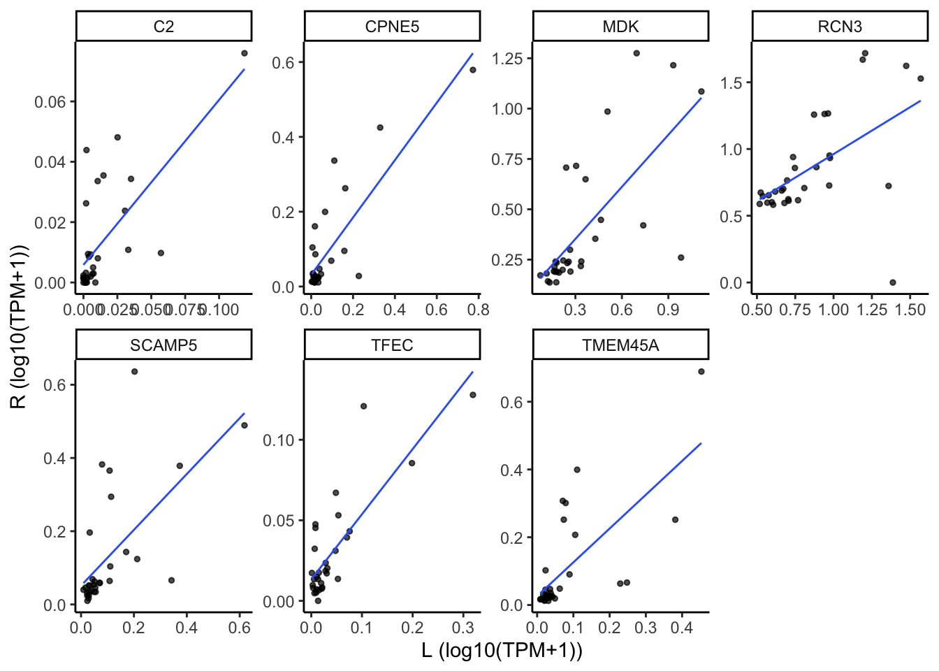
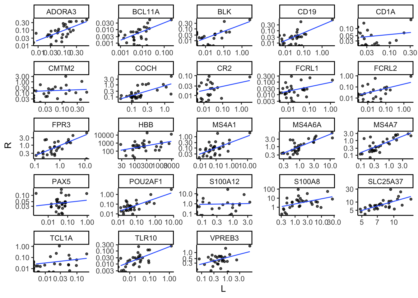
8.6.2 Top loading variables by the PLIER package
In the previou chapter, we employed The PLIER package to estimate the contributions of immune cell types to the FSHD transcriptome. The top Z-loading variables play a crucial role in determining the relative proportions of these immune cell type contributions. Below, we list these top loading variables and their bilateral correlation between L and R biopsies. Please note that they may not necessarily exhibit strong expression levels.
load(file.path(pkg_dir, "data", "plier_topZ_markers.rda"))
markers <- plier_topZ_markers$bilat_markers
gene_cor_topZ <- .markers_bilateral_correlation(markers=markers,
                                           dds=bilat_dds) %>%
    dplyr::left_join(.avg_TPM_by_class(markers = markers, dds=bilat_dds),
                   by="gene_id")

gene_cor_topZ %>%
  dplyr::select(-Pearson_by_TPM) %>%
  kbl(caption="Identified by the PLIER package, listed below are the 18 top Z markers contributed to cell type proportions in bilateral study. The Peason correlation coefficients are compuated using the expression levels presented by Log10(TPM+1).") %>%
kable_styling()| gene_id | gene_name | Pearson_by_log10TPM | LV_index | cell_type | ens_id | Control-like avg TPM | Moderate+ avg TPM | Muscle-Low avg TPM |
|---|---|---|---|---|---|---|---|---|
| ENSG00000110777.12 | POU2AF1 | 0.9220746 | 2,IRIS_Bcell-Memory_IgG_IgA | Bcell-Memory_IgG_IgA | ENSG00000110777 | 0.0312330 | 0.3724736 | 0.1057589 |
| ENSG00000136573.14 | BLK | 0.8141694 | 2,IRIS_Bcell-Memory_IgG_IgA | Bcell-Memory_IgG_IgA | ENSG00000136573 | 0.0108037 | 0.1151240 | 0.0270017 |
| ENSG00000110077.14 | MS4A6A | 0.8063214 | 20,IRIS_DendriticCell-LPSstimulated | DendriticCell-LPSstimulated | ENSG00000110077 | 0.4436241 | 2.1606915 | 3.6416739 |
| ENSG00000177455.15 | CD19 | 0.7963163 | 2,IRIS_Bcell-Memory_IgG_IgA | Bcell-Memory_IgG_IgA | ENSG00000177455 | 0.0199848 | 0.1477995 | 0.0461397 |
| ENSG00000166927.13 | MS4A7 | 0.7842506 | 20,IRIS_DendriticCell-LPSstimulated | DendriticCell-LPSstimulated | ENSG00000166927 | 0.2090296 | 1.1084212 | 1.9491638 |
| ENSG00000132704.16 | FCRL2 | 0.7786763 | 2,IRIS_Bcell-Memory_IgG_IgA | Bcell-Memory_IgG_IgA | ENSG00000132704 | 0.0216208 | 0.1253008 | 0.0336529 |
| ENSG00000282608.2 | ADORA3 | 0.7736084 | 20,IRIS_DendriticCell-LPSstimulated | DendriticCell-LPSstimulated | ENSG00000282608 | 0.0386997 | 0.1584448 | 0.2628639 |
| ENSG00000156738.18 | MS4A1 | 0.6979562 | 2,IRIS_Bcell-Memory_IgG_IgA | Bcell-Memory_IgG_IgA | ENSG00000156738 | 0.0939018 | 0.5551574 | 0.1685982 |
| ENSG00000119866.22 | BCL11A | 0.6909547 | 2,IRIS_Bcell-Memory_IgG_IgA | Bcell-Memory_IgG_IgA | ENSG00000119866 | 0.0025620 | 0.0148748 | 0.0093517 |
| ENSG00000174123.11 | TLR10 | 0.6724404 | 2,IRIS_Bcell-Memory_IgG_IgA | Bcell-Memory_IgG_IgA | ENSG00000174123 | 0.0186041 | 0.0667165 | 0.0748956 |
| ENSG00000147454.14 | SLC25A37 | 0.6618809 | 22,IRIS_Neutrophil-Resting | Neutrophil-Resting | ENSG00000147454 | 6.7495459 | 9.1052736 | 12.1514379 |
| ENSG00000100473.18 | COCH | 0.6310987 | 22,IRIS_Neutrophil-Resting | Neutrophil-Resting | ENSG00000100473 | 0.1073993 | 0.4540094 | 0.9624094 |
| ENSG00000128218.8 | VPREB3 | 0.5787516 | 2,IRIS_Bcell-Memory_IgG_IgA | Bcell-Memory_IgG_IgA | ENSG00000128218 | 0.3698683 | 0.8011012 | 0.5077516 |
| ENSG00000117322.18 | CR2 | 0.5075859 | 2,IRIS_Bcell-Memory_IgG_IgA | Bcell-Memory_IgG_IgA | ENSG00000117322 | 0.0166510 | 0.0830997 | 0.0050237 |
| ENSG00000187474.5 | FPR3 | 0.4933989 | 20,IRIS_DendriticCell-LPSstimulated | DendriticCell-LPSstimulated | ENSG00000187474 | 0.3026753 | 1.7773001 | 1.9219966 |
| ENSG00000158477.7 | CD1A | 0.4457300 | 20,IRIS_DendriticCell-LPSstimulated | DendriticCell-LPSstimulated | ENSG00000158477 | 0.0171722 | 0.0480016 | 0.1425001 |
| ENSG00000244734.4 | HBB | 0.4277861 | 22,IRIS_Neutrophil-Resting | Neutrophil-Resting | ENSG00000244734 | 468.3524397 | 1290.3398086 | 720.0911969 |
| ENSG00000163534.15 | FCRL1 | 0.3398749 | 2,IRIS_Bcell-Memory_IgG_IgA | Bcell-Memory_IgG_IgA | ENSG00000163534 | 0.0200861 | 0.0731329 | 0.0216181 |
| ENSG00000143546.10 | S100A8 | 0.3275266 | 22,IRIS_Neutrophil-Resting | Neutrophil-Resting | ENSG00000143546 | 4.3832407 | 7.8536112 | 3.5999534 |
| ENSG00000196092.14 | PAX5 | 0.3205516 | 2,IRIS_Bcell-Memory_IgG_IgA | Bcell-Memory_IgG_IgA | ENSG00000196092 | 0.0535907 | 0.0706754 | 0.0370464 |
| ENSG00000140932.10 | CMTM2 | 0.2400213 | 22,IRIS_Neutrophil-Resting | Neutrophil-Resting | ENSG00000140932 | 0.1152954 | 0.2188711 | 0.2500067 |
| ENSG00000163221.9 | S100A12 | 0.2350988 | 22,IRIS_Neutrophil-Resting | Neutrophil-Resting | ENSG00000163221 | 0.6872278 | 1.6299728 | 0.6324510 |
| ENSG00000100721.11 | TCL1A | 0.2112394 | 22,IRIS_Neutrophil-Resting | Neutrophil-Resting | ENSG00000100721 | 0.0296388 | 0.0680252 | 0.0049452 |
write_xlsx(list(`63 immune-cell-markers`= gene_cor_63,
                `23 top loading variables (PLIER)`=gene_cor_topZ),
           path=file.path(pkg_dir, "stats",
          "Bilateral-correlation-63-immune-cell-markers-and-23-topZ-by-PLIER.xlsx"))
Check the scatter plot: TPM on x and y coordinates are displayed in log10 scale.