10 Complement scoring
The complement scoring was obtained from the file /extdata-github/FINAL.Revised.BilatStudy.Path.MACstaining data.FINAL.xlsx. The scoring system quantifies the MAC staining into four levels:
- Absence of MAC staining in capillaries
- Slight level of MAC staining
- Moderate levet of MAC staining
- Prominent level of MAC staining
Note that no bilateral sample was identified as level 4
library(tidyverse)
library(corrr)
pkg_dir <- "/Users/cwon2/CompBio/Wellstone_BiLateral_Biopsy"
load(file.path(pkg_dir, "data", "comprehensive_df.rda"))
10.1 Complement scoring (MCA score) and basket scores
Here, we investigated the relationship between the complement scoring and the basket scores.
Result:
- The complement scoring has moderate correlation with basket scores. The code chunk below calculates the Spearman correlation coefficients.
- ANOVA p-values reveals significant difference of the mean values of basket score in three levels of complement scoring.
10.1.1 Correlation with basekt scores
The complement scoring has moderate correlation with basket scores. The code chunk below calculates the Spearman correlation coefficients.
# get complement scoring and basekt scores from  `comprehensive_df`
df <- comprehensive_df %>%
  drop_na(`Complement Scoring`, `IG-logSum`) %>%
  dplyr::select(`Complement Scoring`, `DUX4-M6-logSum`,
                `IG-logSum`, `Complement-logSum`,
                `Inflamm-logSum`, `ECM-logSum`)

  #dplyr::mutate(`Complement Scoring` = factor(`Complement Scoring`))
df %>%
  corrr::correlate(., method="spearman") %>%
  dplyr::select(term, `Complement Scoring`) %>%
  dplyr::filter(term != "Complement Scoring") %>%
  dplyr::rename(basket = term) %>%
  dplyr::mutate(basket = str_replace(basket, "-logSum", ""))
#> # A tibble: 5 × 2
#>   basket     `Complement Scoring`
#>   <chr>                     <dbl>
#> 1 DUX4-M6                   0.542
#> 2 IG                        0.509
#> 3 Complement                0.453
#> 4 Inflamm                   0.452
#> 5 ECM                       0.452
10.1.2 Visualize the relationship with basket scores
# tidy up the data.frame for visualization
tidy_df <- df %>%
  dplyr::mutate(`Complement Scoring` = factor(`Complement Scoring`)) %>%
  tidyr::gather(key=`basket`, value=`basket score`,
                -`Complement Scoring`) %>%
  dplyr::mutate(basket = str_replace(basket, "-logSum", "")) %>%
  dplyr::mutate(`Complement Scoring` = factor(`Complement Scoring`),
                basket = factor(basket,
                                levels=c("DUX4-M6", "ECM", "Inflamm",
                                         "Complement", "IG")))
Display dotplot with color:
ggplot(tidy_df, aes(x=`Complement Scoring`, y=`basket score`)) +
    geom_dotplot(aes(fill=`Complement Scoring`,
                     color=`Complement Scoring`),
                 binaxis='y', stackdir='center',
                 show.legend = FALSE,
                 stackratio=1.5, dotsize=1.5) +
    stat_summary(fun.data=mean_sdl, fun.args = list(mult=1),
                 geom="pointrange", color="red", fill="red", shape=23,
                 size=0.5, alpha=0.5) +
    facet_wrap(~basket, scales="free_y") +
    scale_fill_brewer(palette="Blues") +
    scale_color_brewer(palette="Blues") +
    theme_classic() + labs(x="complement scoring")
ANOVA p-values of the mean value differences of basket scores among three leves of complemnt scoring.
tm <- tidy_df %>% group_by(basket) %>%
  dplyr::do(aov = summary(aov(`basket score` ~ `Complement Scoring`,
                             data = .)))
names(tm$aov) <- levels(tidy_df$basket)
tm$aov
#> $`DUX4-M6`
#>                      Df Sum Sq Mean Sq F value   Pr(>F)
#> `Complement Scoring`  2  46.78  23.390   11.13 8.31e-05 ***
#> Residuals            57 119.80   2.102
#> ---
#> Signif. codes:
#> 0 '***' 0.001 '**' 0.01 '*' 0.05 '.' 0.1 ' ' 1
#>
#> $ECM
#>                      Df Sum Sq Mean Sq F value   Pr(>F)
#> `Complement Scoring`  2  74.48   37.24   11.07 8.66e-05 ***
#> Residuals            57 191.70    3.36
#> ---
#> Signif. codes:
#> 0 '***' 0.001 '**' 0.01 '*' 0.05 '.' 0.1 ' ' 1
#>
#> $Inflamm
#>                      Df Sum Sq Mean Sq F value Pr(>F)
#> `Complement Scoring`  2  51.29  25.646   9.385  3e-04 ***
#> Residuals            57 155.77   2.733
#> ---
#> Signif. codes:
#> 0 '***' 0.001 '**' 0.01 '*' 0.05 '.' 0.1 ' ' 1
#>
#> $Complement
#>                      Df Sum Sq Mean Sq F value   Pr(>F)
#> `Complement Scoring`  2  78.44   39.22   9.423 0.000291 ***
#> Residuals            57 237.23    4.16
#> ---
#> Signif. codes:
#> 0 '***' 0.001 '**' 0.01 '*' 0.05 '.' 0.1 ' ' 1
#>
#> $IG
#>                      Df Sum Sq Mean Sq F value   Pr(>F)
#> `Complement Scoring`  2  295.5  147.77   17.56 1.14e-06 ***
#> Residuals            57  479.6    8.41
#> ---
#> Signif. codes:
#> 0 '***' 0.001 '**' 0.01 '*' 0.05 '.' 0.1 ' ' 1
10.2 Complement Scoring correlation between left and right biopsies
Out of 34 subject 29 have complement scoring on both left and right biopsies. We aim to evalulate the correlation between left and right.
10.3 Complement Scoring vs. STIR status
The average complement scoring for STIR- and STIR+ samples are 1.38 (+/-0.63SD) and 2.08 (+/-0.929SD), respectively.
comprehensive_df %>%
  drop_na(`Complement Scoring`, `STIR_status`) %>%
  group_by(STIR_status) %>%
  summarize(mean=mean(`Complement Scoring`),
            sd = sd(`Complement Scoring`)) %>%
  ggplot(aes(x=STIR_status, y=`mean`)) +
  geom_bar(stat="identity",fill="skyblue", alpha=0.7,
           position=position_dodge()) +
  geom_errorbar(aes(ymin=mean-sd, ymax=mean+sd), width=0.4,
                 position=position_dodge(.9),
                colour="orange", alpha=0.9, linewidth=1.5) +
  theme_minimal() +
  theme(panel.grid.major = element_blank()) +
  labs(y="Complement Scoring", x="")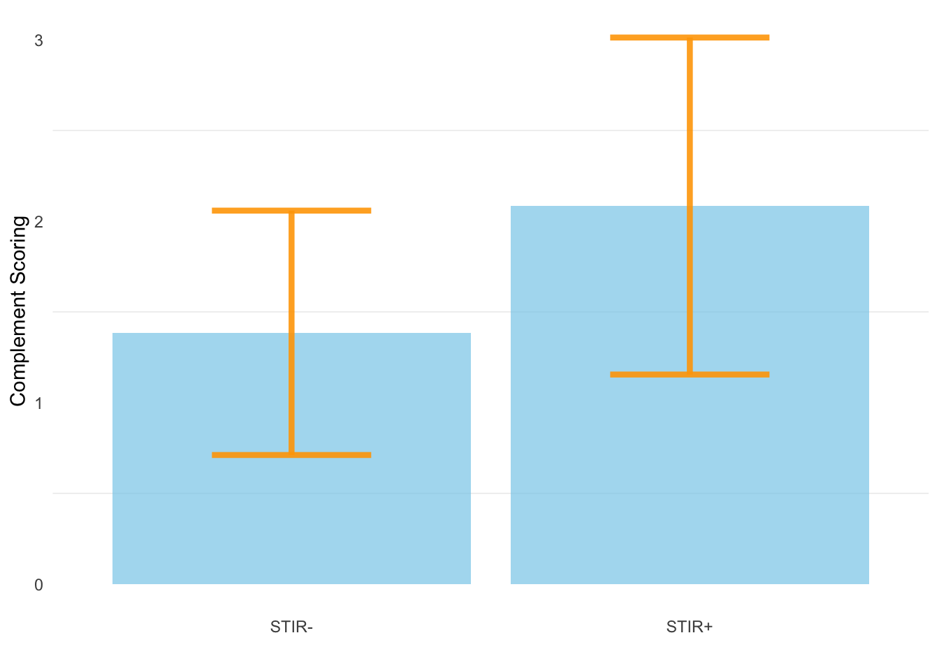
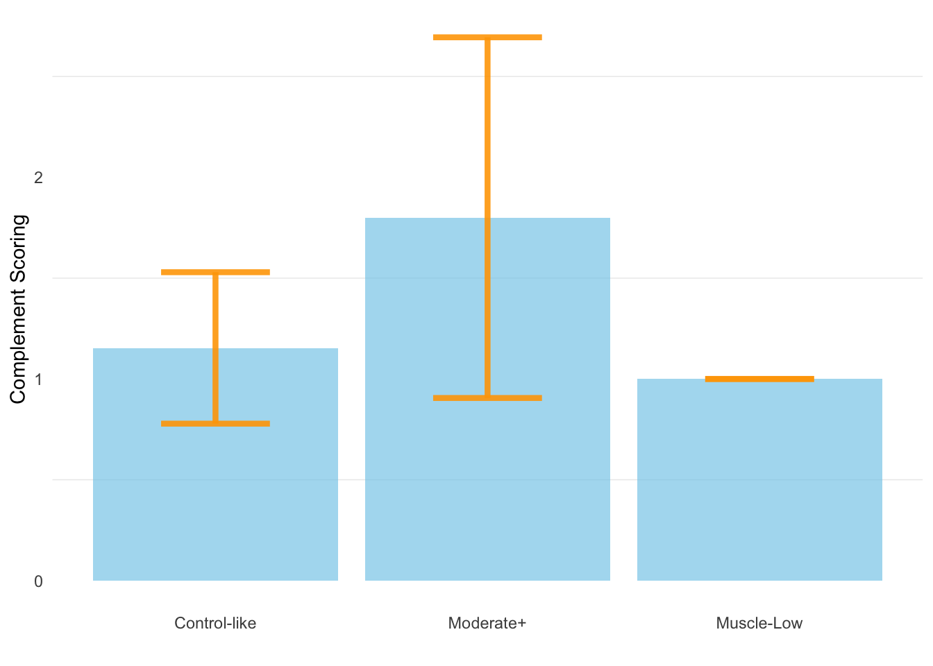
10.4 Complement scoring vs. class
The average complement scoring for Control-like, Moderate+, and Muscle-Low samples are 1.15 (+- 0.376SD), 1.8 (+/- 0.894SD), and 1, respectively.
comprehensive_df %>%
  drop_na(`Complement Scoring`, `class`) %>%
  dplyr::select(`Complement Scoring`, `class`) %>%
  group_by(class) %>%
  summarize(mean=mean(`Complement Scoring`),
            sd = sd(`Complement Scoring`)) %>%
  ggplot(aes(x=class, y=`mean`)) +
  geom_bar(stat="identity",fill="skyblue", alpha=0.7,
           position=position_dodge()) +
  geom_errorbar(aes(ymin=mean-sd, ymax=mean+sd), width=0.4,
                 position=position_dodge(.9),
                colour="orange", alpha=0.9, linewidth=1.5) +
  theme_minimal() +
  theme(panel.grid.major = element_blank()) +
  labs(y="Complement Scoring", x="")