9 Immune cell type proportion by PLIER
The PLIER package1 provides an alternative to examine the immune cell infiltration, without involving in GO or differential analysis as we have investigated in @ref{immune-cell-infiltrates}. PLIER employes eigenvalue-like decomposition to estimate the immune cell contribution to the FSHD transcriptome. The top loading variables from the resulting eigenvalue-like latent variables (LV) are potential indicators of immune infiltrate signatures. We utilized the PLIER algorithm for analyzing both longitudinal and bilateral samples. The expression levels of the most influential loading variables are depicted in this chapter.
# define parameters and load datasets: bilat_dds and longitudinal_dds
pkg_dir <- "/Users/cwon2/CompBio/Wellstone_BiLateral_Biopsy"
fig_dir <- file.path(pkg_dir, "figures", "immune-infiltration")
source(file.path(pkg_dir, "scripts", "load_variables_and_datasets.R"))
# returns bilat_dds and longitudinal_dds
We ultitized the IRIS dataset2 from PLIER as the baseline of immnune cell types and markers.
library(PLIER)
data(bloodCellMarkersIRISDMAP)
# Extract the IRIS dataset from `bloodCellMarkersIRISDMAP`
blood_iris <- as.data.frame(bloodCellMarkersIRISDMAP) %>%
  rownames_to_column(var="gene_name") %>%
  dplyr::select(gene_name, starts_with("IRIS")) %>%
  dplyr::filter(rowSums(across(where(is.numeric))) > 0)

bilat_coldata <- colData(bilat_dds) %>% as.data.frame()
longi_coldata <- colData(longitudinal_dds) %>% as.data.frame()
9.1 PLIER Longitudinal samples
In this section, we applied PLIER to estimate the immune cell type proportion for the longitudiname samples.
9.1.1 Steps
- run PLIER, the
priorMatonly includes the IRIS dataset (blood_iris) - Select top LVs with AUC > 0.8 and FDR < 0.05
- Verify the top LVs of elevated proportion in FSHD and filter out the false positives
- Identify top loading varibles associated with the selected top LVs
# use RPKM as suggested by the PLIER authers; TPM yields similar results
longitudinal_rpkm <- assays(longitudinal_dds)[["RPKM"]]
longitudinal_tpm <- assays(longitudinal_dds)[["TPM"]]
rownames(longitudinal_rpkm) <-
  rownames(longitudinal_tpm) <- rowData(longitudinal_dds)$gene_name

priorMat <-
  bloodCellMarkersIRISDMAP[, names(blood_iris)[-1]] # remove col "gene_name"
plier_longi <- PLIER(longitudinal_rpkm, # or longitudinal_rpkm
                     priorMat=priorMat,
                     scale = TRUE)
#> [1] 24.90828
#> [1] "L2 is set to 24.908276840206"
#> [1] "L1 is set to 12.454138420103"
mat_u <- plotU(plier_longi, auc.cutoff = 0.70, fdr.cutoff = 0.05, top = 3)
Figure 9.1: Significant LVs with AUC > 0.8 and FDR < 0.05.
sig_sets <- names(mat_u$iirow)[mat_u$iirow]Displayed below is the visualization of eight latent variables (LVs) that potentially capture the immune cell infiltrate signatures in the more affected muscles. It is important to note that there may be some false positives among them.
# proportion boxplots of all the sig LVs
sig_proportion_longi <- plier_longi$B[mat_u$iicol, ] %>% as.data.frame() %>%
  rownames_to_column(var="LV_index") %>%
  tidyr::gather(key=sample_id, value=proportion, -LV_index) %>%
  left_join(dplyr::select(longi_coldata, sample_id, cluster), by="sample_id")

outliers <- sig_proportion_longi %>% dplyr::filter(proportion > 3)

sig_proportion_longi %>%
    dplyr::filter(proportion < 3) %>%
ggplot(aes(x=cluster, y=proportion)) +
  geom_boxplot(width=0.3, outlier.shape = NA) +
  geom_jitter(width=0.3, size=0.3, color="grey50") +
  facet_wrap(~LV_index, scale="free_y", ncol=3) +
  theme_minimal() +
  theme(axis.text.x = element_text(angle = 90, vjust = 0.5, hjust=1),
        axis.title.x = element_blank(),
        panel.grid.major = element_blank(), panel.grid.minor = element_blank())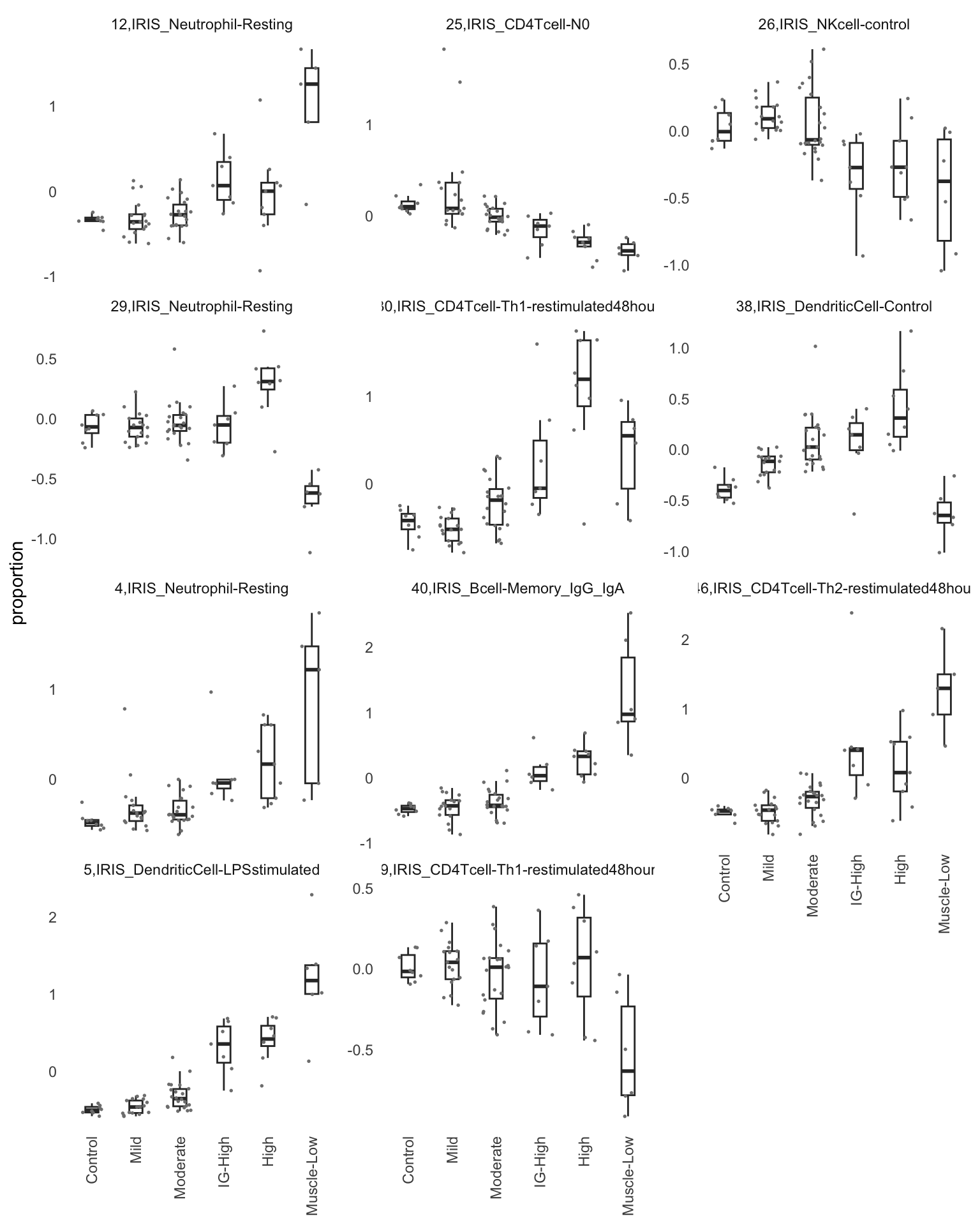
Figure 9.2: The cell type proportion of all significant LVs
9.1.2 Five best LVs showing immune cell infiltrat signatures
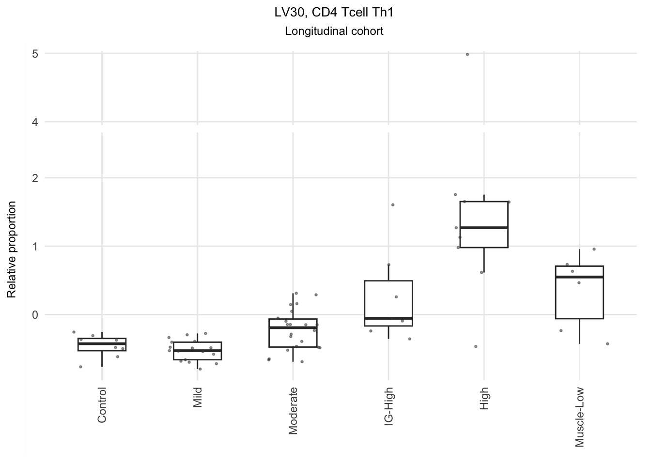
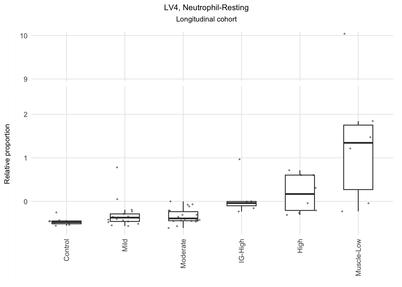
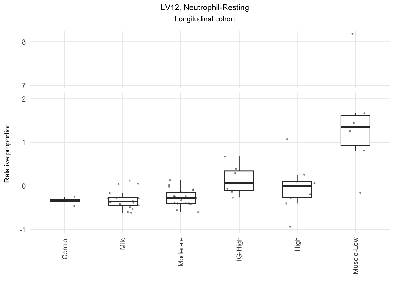
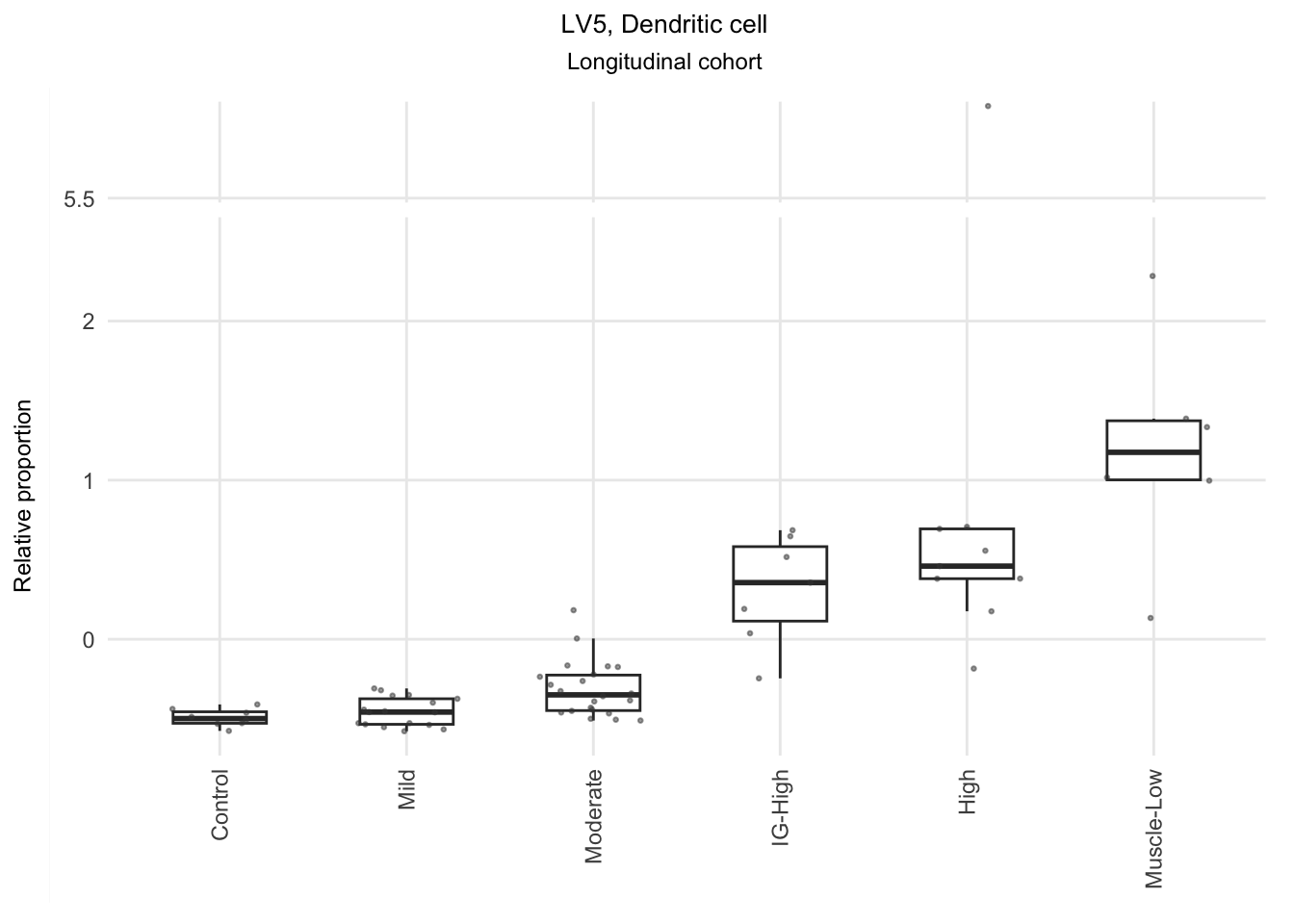
Based on the information extracted from the U, top Z, and B matrices, it can be concluded that LV30, LV4, LV5, LV12, and LV46 are the most reliable latent variables indicating heightened immune cell infiltration. Consequently, we have generated plots for our publication showcasing the following latent variables: LV30 (CD4 Tcell-Th1), LV4 and LV12 (Neutrophil resting), LV40 (IgG and IgA B memory cell), and LV5 (dendritic cell).
NOTE: I hide the code chuck for they are tidious, but the reader cand find them in the original Rmd files.

9.1.3 Top loading variables Z of selected LVs
LV_index<- c(4, 5, 12, 30, 40)
names(LV_index) <- rownames(plier_longi$B[LV_index, ])
priorMat <- bloodCellMarkersIRISDMAP[, names(blood_iris)[-1]]

top = 15
sub_iris <- blood_iris %>%
  dplyr::select(gene_name, `IRIS_CD4Tcell-Th1-restimulated48hour`,
                `IRIS_CD4Tcell-Th2-restimulated48hour`,
                `IRIS_DendriticCell-Control`,
                `IRIS_DendriticCell-LPSstimulated`,
                `IRIS_CD4Tcell-Th2-restimulated12hour`,
                `IRIS_Bcell-Memory_IgG_IgA`,
                `IRIS_Neutrophil-Resting`)

longi_topZ <- map_dfr(LV_index, function(index) {
  plier_longi$Z[, index, drop=FALSE] %>% as.data.frame() %>%
    arrange(-V1) %>% top_n(top) %>%
    dplyr::select(-V1) %>%
    #dplyr::rename_with(~paste0("LV", as.character(index))) %>%
    rownames_to_column(var="gene_name") %>%
    left_join(sub_iris, by="gene_name") %>% # turn NA to 0
    replace(is.na(.), 0) %>%
    dplyr::mutate(in_markerSet =
                    if_else(rowSums(across(where(is.numeric))) > 0,
                                    TRUE, FALSE), .after=gene_name)
    # which pathway?
}, .id="LV_index") %>% # append gene_id
  left_join(anno_ens88, by="gene_name") %>%
  left_join(dplyr::select(anno_gencode35, gencode35_id, gene_name),
            by="gene_name")
longi_topZ %>% group_by(LV_index) %>%
  summarize(n=sum(in_markerSet)) %>%
  knitr::kable(format = "html",
caption="The five most reliable LVs and the number of top loading variables associated with the LVs.")| LV_index | n |
|---|---|
| 12,IRIS_Neutrophil-Resting | 7 |
| 30,IRIS_CD4Tcell-Th1-restimulated48hour | 7 |
| 4,IRIS_Neutrophil-Resting | 11 |
| 40,IRIS_Bcell-Memory_IgG_IgA | 13 |
| 5,IRIS_DendriticCell-LPSstimulated | 4 |
The code chunk below tidied up the top loading variables and attached annotation.
longi_topZ <- longi_topZ %>%
  dplyr::mutate(cell_type = str_replace(LV_index, "[0-9]*,IRIS_", ""))

longi_markers <- map_dfr(names(LV_index), function(lv) {
  longi_topZ %>% dplyr::filter(LV_index == lv, in_markerSet) %>%
    dplyr::select(LV_index, cell_type, ens_id)
}) %>% dplyr::arrange(cell_type) %>%
  left_join(dplyr::select(anno_ens88, ens88_id, ens_id, gene_name),
            by="ens_id") %>%
  dplyr::rename(gene_id = ens88_id)
9.1.3.1 Heatmap of top loading variables
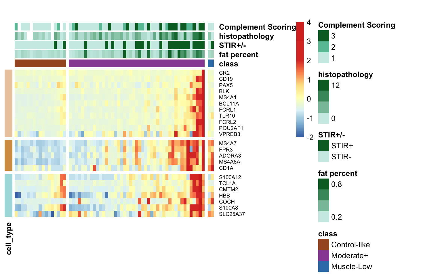
Below is the heatmap illustrating the z-scores of the log TPM (transcripts per million) values for the top loading variables associated with the five latent variables (LVs).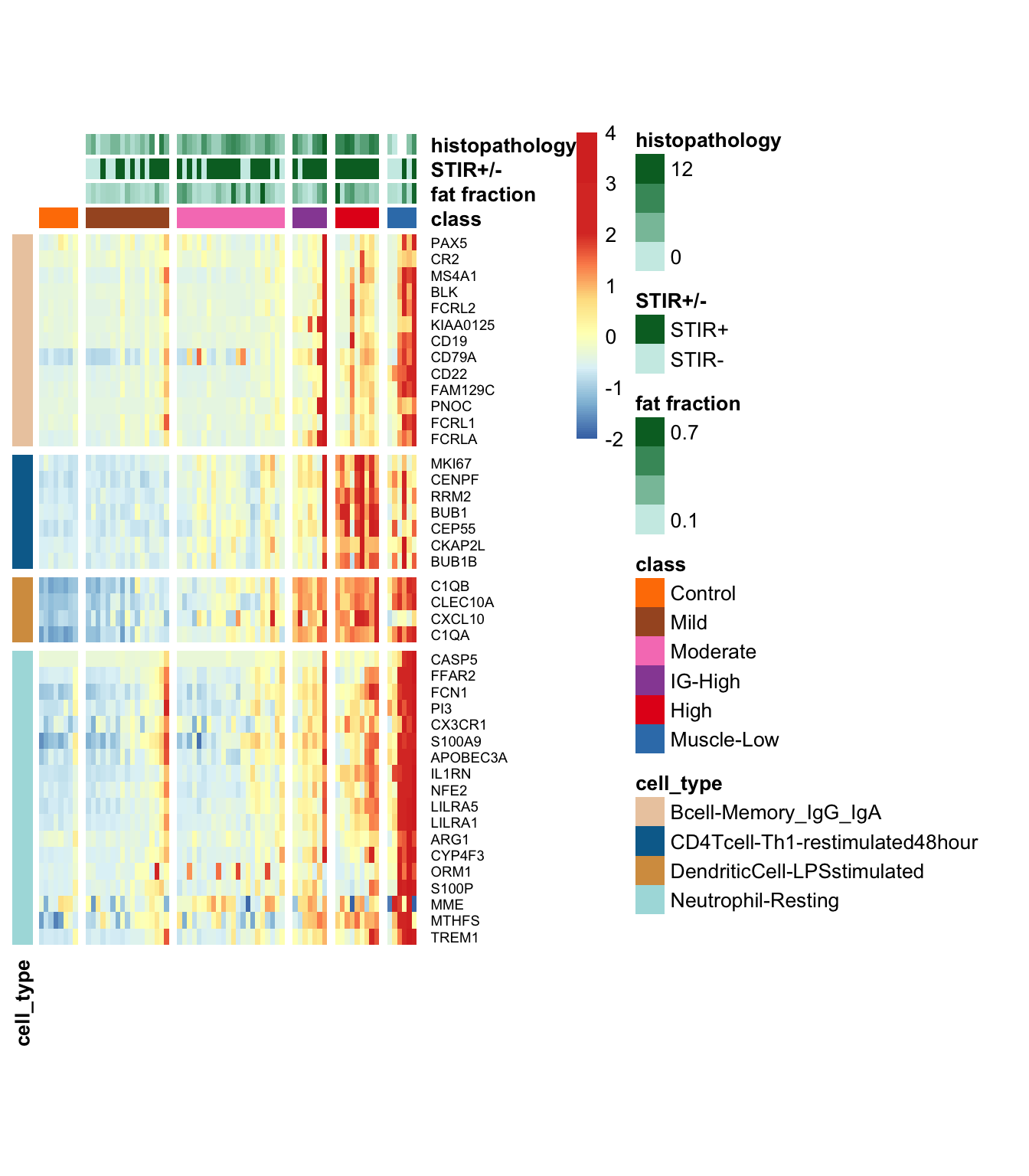
Figure 9.3: Heatmap of the top loading variables associated with the five LVs for longitudinal samples.
9.2 PLIER to the bilateral samples
We applied PLIER to the bilateral samples in the same matter. The cut off values for LVs are : AUC = 0.7 and FDR = 0.05
bilat_rpkm <- assays(bilat_dds)[["RPKM"]]
bilat_tpm <- assays(bilat_dds)[["TPM"]]

rownames(bilat_rpkm) <- rownames(bilat_tpm) <- rowData(bilat_dds)$gene_name
plier_bilat <- PLIER(bilat_rpkm, # or longitudinal_rpkm
                     priorMat=priorMat,
                     scale = TRUE)
#> [1] 29.88863
#> [1] "L2 is set to 29.8886299733202"
#> [1] "L1 is set to 14.9443149866601"
save(plier_bilat, file=file.path(pkg_dir, "data", "plier_bliat.rda"))
mat_u <- plotU(plier_bilat, auc.cutoff = 0.7, fdr.cutoff = 0.05, top = 3)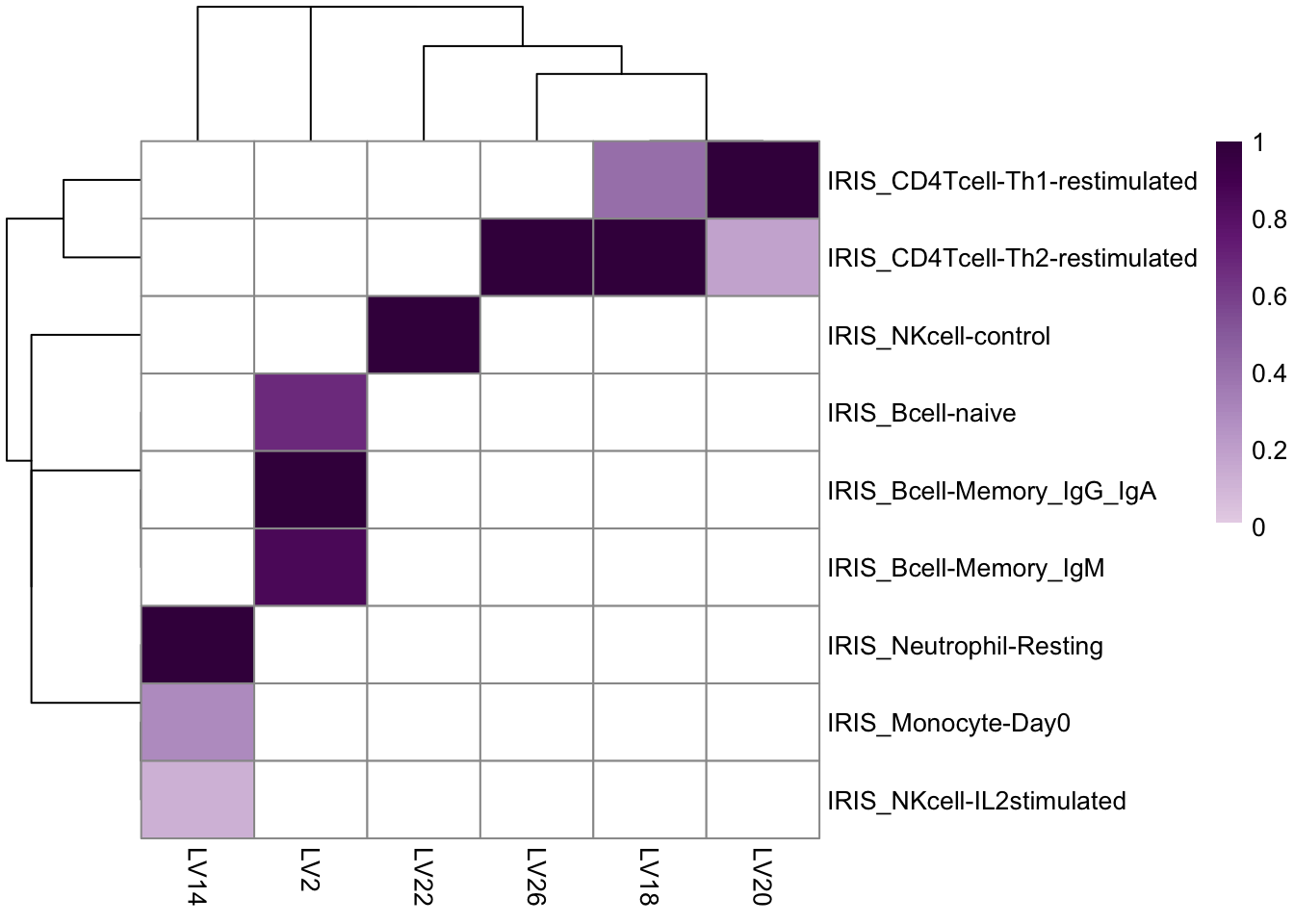
bilat_col_data <- colData(bilat_dds) %>% as.data.frame()

# define sig LV_index:
LV_index <- c(2, 14, 18, 20, 26, 22)
names(LV_index) <- rownames(plier_bilat$B[LV_index, ])

#plier_bilat$B[LV_index, ] %>% as.data.frame() %>%
#  rownames_to_column(var="LV_index") %>%
#  tidyr::gather(key=sample_id, value=proportion, -LV_index) %>%
#  left_join(dplyr::select(bilat_col_data, sample_id, class), by="sample_id") %>%
#  dplyr::filter(proportion >= 3) %>%
#  knitr::kable(caption="Samples with extreme proportions. Remov ed from the #figure below.")

# boxplot for proportion of potential LVs
plier_bilat$B[mat_u$iicol, ] %>% as.data.frame() %>%
  rownames_to_column(var="LV_index") %>%
  tidyr::gather(key=sample_id, value=proportion, -LV_index) %>%
  left_join(dplyr::select(bilat_col_data, sample_id, class), by="sample_id") %>%
  dplyr::filter(proportion < 3) %>%
  ggplot(aes(x=class, y=proportion)) +
    geom_boxplot(width=0.3, outlier.shape = NA) +
    geom_jitter(width=0.3, size=0.3) +
    facet_wrap(~LV_index, scale="free_y", nrow=3) +
    #labs(title="Remove outliers with proportion > 3 ") +
    theme_minimal() +
    theme(axis.text.x = element_text(angle = 90, vjust = 0.5, hjust=1),
          axis.title.x = element_blank())
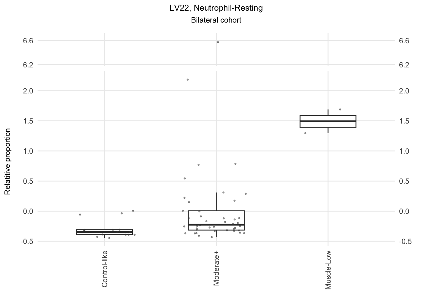
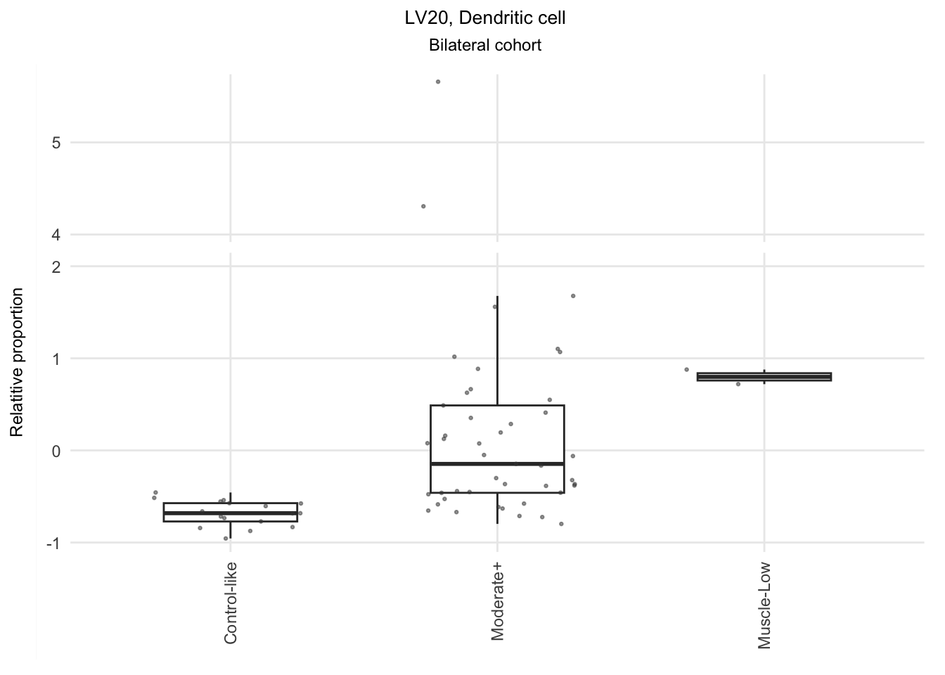
9.2.1 Three base LVs demonstrating elevated immune cell proportion
The significant LVs that show elevated immune cell type contribution in FSHD are LV2 (Bcell-Memory_IgG_IgA), LV22 (Neutrophil-resting) and LV20 (DendriticCell-LPSstimulated). LV18 and LV26 do have elevated proportion in moderatedly-affected muscles.
bilat_proportion <- plier_bilat$B[LV_index, ] %>% as.data.frame() %>%
  rownames_to_column(var="LV_index") %>%
  tidyr::gather(key=sample_id, value=proportion, -LV_index) %>%
left_join(dplyr::select(bilat_col_data, sample_id, class), by="sample_id") 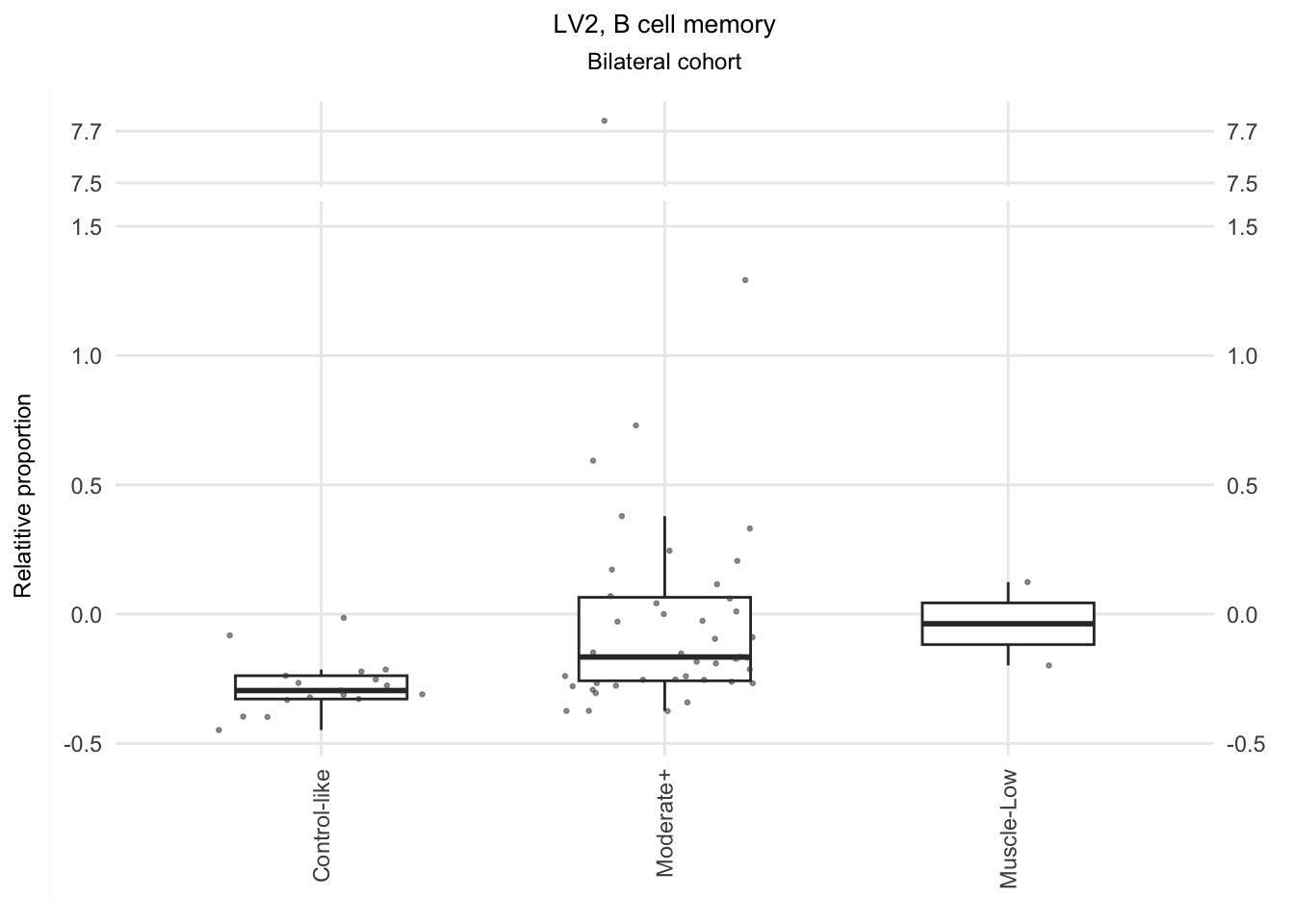
9.2.1.4 Top loading variables (Z) of selected LVs
bilat_LV <- c(2, 20, 22)
names(bilat_LV) <- rownames(plier_bilat$B[bilat_LV, ])
priorMat <- bloodCellMarkersIRISDMAP[, names(blood_iris)[-1]]

top = 15
sub_iris <- blood_iris %>%
  dplyr::select(gene_name, `IRIS_CD4Tcell-Th1-restimulated48hour`,
                `IRIS_CD4Tcell-Th2-restimulated48hour`,
                `IRIS_Bcell-Memory_IgG_IgA`, `IRIS_Bcell-naive`,
                `IRIS_Bcell-naive`, `IRIS_Bcell-Memory_IgM`,
                `IRIS_Neutrophil-Resting`,
                `IRIS_DendriticCell-Control`,
                `IRIS_DendriticCell-LPSstimulated`)

bilat_topZ <- map_dfr(bilat_LV, function(index) {
  plier_bilat$Z[, index, drop=FALSE] %>% as.data.frame() %>%
    arrange(-V1) %>% top_n(top) %>%
    dplyr::select(-V1) %>%
    #dplyr::rename_with(~paste0("LV", as.character(index))) %>%
    rownames_to_column(var="gene_name") %>%
    left_join(sub_iris, by="gene_name") %>% # turn NA to 0
    replace(is.na(.), 0) %>%
    dplyr::mutate(in_markerSet =
                    if_else(rowSums(across(where(is.numeric))) > 0,
                                    TRUE, FALSE), .after=gene_name)
}, .id="LV_index") %>% # append gene_id
  left_join(anno_ens88, by="gene_name") %>%
  left_join(dplyr::select(anno_gencode35, gencode35_id, gene_name),
            by="gene_name")
#top_z <- bilat_topZ
bilat_topZ %>% group_by(LV_index) %>%
  summarize(n=sum(in_markerSet)) %>%
knitr::kable(caption="The three best LVs and the number of associated makers.")| LV_index | n |
|---|---|
| 2,IRIS_Bcell-Memory_IgG_IgA | 11 |
| 20,IRIS_DendriticCell-LPSstimulated | 5 |
| 22,IRIS_Neutrophil-Resting | 7 |
#bilat_LV <- c(2, 20, 22)
#names(bilat_LV) <- rownames(plier_bilat$B[bilat_LV, ])
bilat_topZ <- bilat_topZ %>%
    dplyr::mutate(cell_type = str_replace(LV_index, "[0-9]*,IRIS_", ""))

bilat_markers <-  map_dfr(names(bilat_LV), function(lv) {
  bilat_topZ %>% dplyr::filter(LV_index == lv, in_markerSet) %>%
    dplyr::select(LV_index, cell_type, ens_id)
}) %>% dplyr::arrange(cell_type) %>%
   left_join(dplyr::select(anno_gencode35, gencode35_id, ens_id, gene_name),
            by="ens_id") %>%
    dplyr::rename(gene_id = gencode35_id)